Plot the output from a geostatistical model of survey data

Takes the output from fit_survey_sets() and creates a map of the model predictions and/or the raw data. Includes a number of options for customizing the map including the ability to rotate the map.

plot_survey_sets(pred_dat, raw_dat, fill_column = c("combined", "bin",
  "pos"), fill_scale = ggplot2::scale_fill_viridis_c(trans = "sqrt",
  option = "C"), colour_scale = ggplot2::scale_colour_viridis_c(trans =
  "sqrt", option = "C"), pos_pt_col = "#FFFFFF60",
  bin_pt_col = "#FFFFFF40", pos_pt_fill = "#FFFFFF05",
  pt_size_range = c(0.5, 9), show_legend = TRUE,
  extrapolate_depth = TRUE, extrapolation_buffer = 0,
  show_model_predictions = TRUE, show_raw_data = TRUE, utm_zone = 9,
  fill_label = "Predicted\nbiomass\ndensity (kg/m^2)",
  pt_label = "Tow density (kg/km^2)", rotation_angle = 0,
  rotation_center = c(500, 5700), show_axes = TRUE, xlim = NULL,
  ylim = NULL, x_buffer = c(-5, 5), y_buffer = c(-5, 5),
  north_symbol = FALSE, north_symbol_coord = c(130, 5975),
  north_symbol_length = 30, cell_size = 2, circles = FALSE)

Arguments

pred_dat	The predictions element of the output from fit_survey_sets().
raw_dat	The data element of the output from fit_survey_sets().
fill_column	The name of the column to plot. Options are "combined" for the combined model, "bin" for the binary component model, or "pos" for the positive component model.
fill_scale	A ggplot scale_fill_* object.
colour_scale	A ggplot scale_colour_* object. You likely want this to match fill_scale unless you want the map to look strange.
pos_pt_col	The color for positive set location points.
bin_pt_col	The color for binary set location points.
pos_pt_fill	The fill color for positive set location points.
pt_size_range	The range of point sizes for positive set location points.
show_legend	Logical for whether or not to show the legend.
extrapolate_depth	Logical for whether or not to show predictions across all depths in the survey domain (the default) or to not extrapolate beyond the range of the observed sets in the data set.
extrapolation_buffer	A buffer to add to the minimum and maximum observed depths if extrapolate_depth = TRUE.
show_model_predictions	Logical for whether or not to show the geostatistical model predictions.
show_raw_data	Logical for whether or not to show the raw data.
utm_zone	The UTM zone to plot in. Should match the zone used in fit_survey_sets().
fill_label	A label to use in the legend for the fill color.
pt_label	A label to use in the legend for the point size.
rotation_angle	An angle to rotate the entire map. Can be useful to make a map of the BC coast take up less. Defaults to not rotating the map. The groundfish synopsis report uses rotation_angle = 40.
rotation_center	The coordinates around which to rotate the mouth. These should be in UTM coordinates.
show_axes	Logical for whether or not to show the axes.
xlim	X axis limits in UTM coordinates. The synopsis report uses c(360, 653). Defaults to the range of the data.
ylim	Y axis limits in UTM coordinates. The synopsis report uses c(5275, 6155). Defaults to the range of the data.
x_buffer	A buffer in UTM coordinates to extend the X axis. Mostly useful if the axis limits aren't explicitly specified.
y_buffer	A buffer in UTM coordinates to extend the Y axis. Mostly useful if the axis limits aren't explicitly specified.
north_symbol	Logical for whether to include a north symbol.
north_symbol_coord	Coordinates for the north symbol in UTM coordinates.
north_symbol_length	Length of the north assemble arrow.
cell_size	The size of the grid cells for the model predictions.
circles	Logical for whether to plot the model predictions in circles. This analysis report uses this for the IPHC survey.

Value

A ggplot object.

Examples

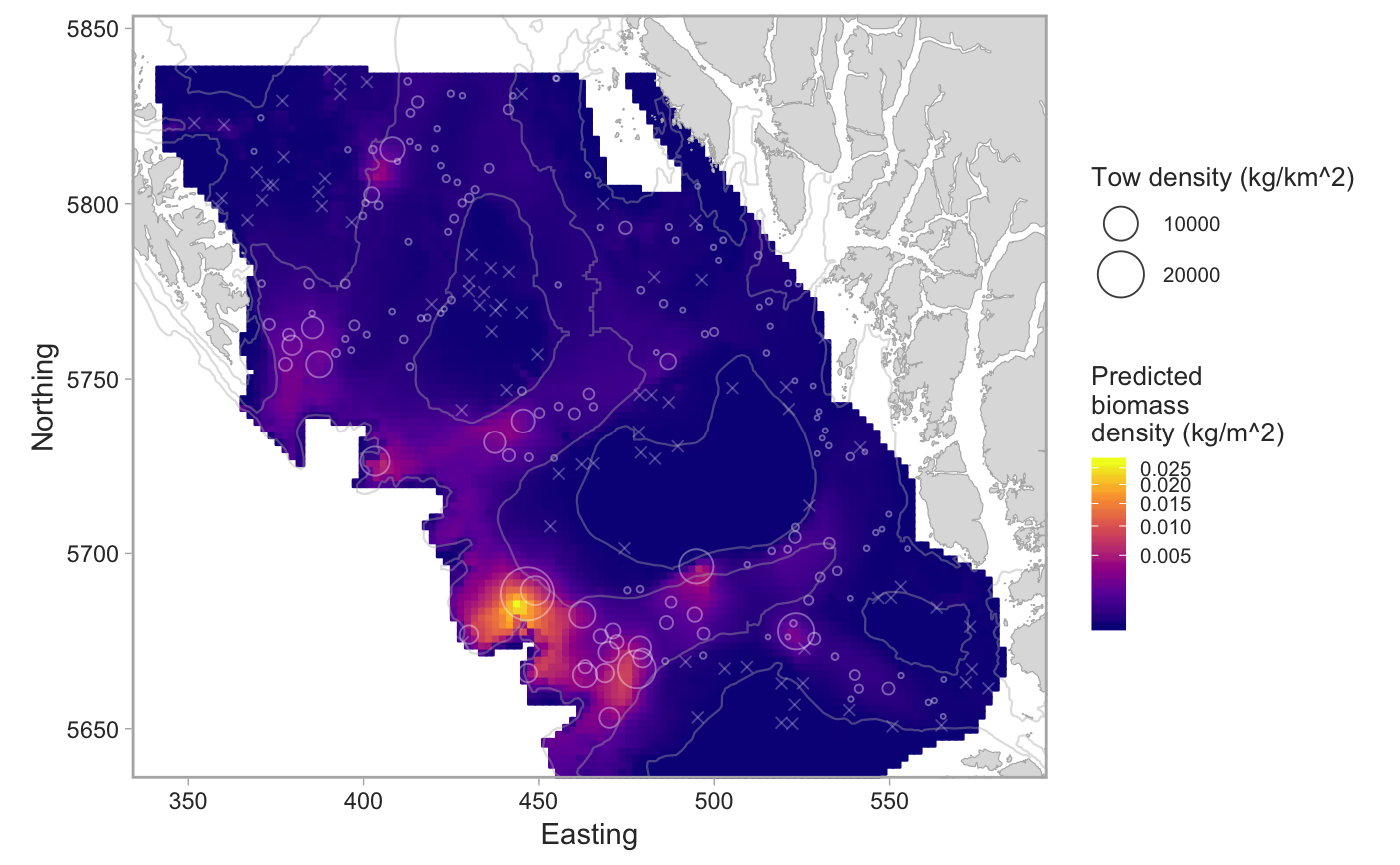
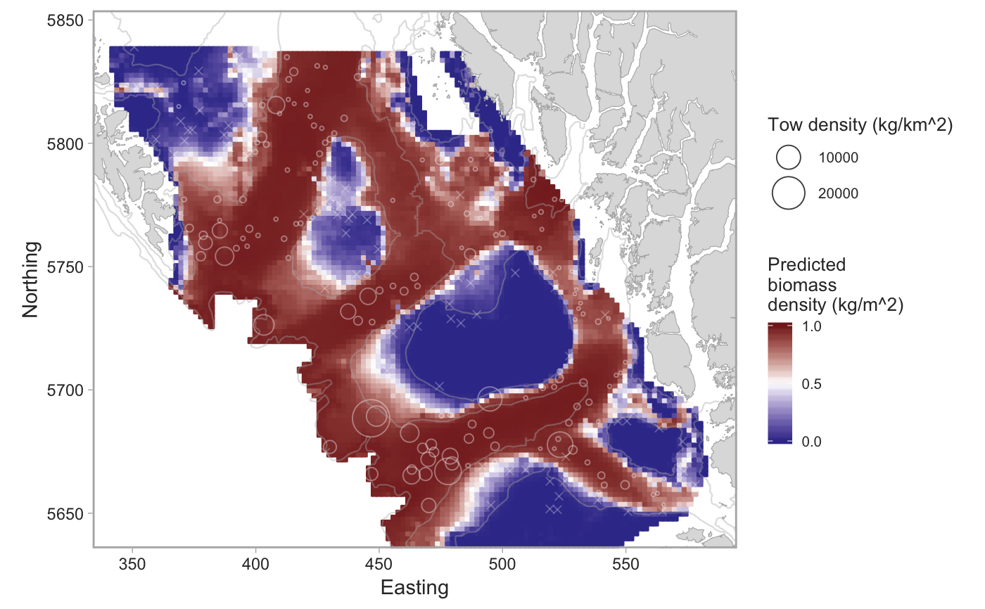
set.seed(123)
# pop_surv <- get_survey_sets("pacific ocean perch")
# or use built-in data:
fit <- fit_survey_sets(pop_surv,
  years = 2015,
  survey = "SYN QCS")
#> Preloading interpolated depth for prediction grid...
#> Predicting density onto grid...
#> INLA max_edge = c(20, 100)
#> INLA max_edge = c(20, 100)

# The combined model:
plot_survey_sets(fit$predictions, fit$data, fill_column = "combined")
# The positive component model:
plot_survey_sets(fit$predictions, fit$data, fill_column = "pos")
# Add a custom color scale for the binary model:
plot_survey_sets(fit$predictions, fit$data, fill_column = "bin") +
  ggplot2::scale_fill_gradient2(midpoint = 0.5,
    high = scales::muted("red"),
    mid = "white",
    low = scales::muted("blue"), limits = c(0, 1), breaks = c(0, 0.5, 1)) +
  ggplot2::scale_colour_gradient2(midpoint = 0.5,
    high = scales::muted("red"),
    mid = "white",
    low = scales::muted("blue"), limits = c(0, 1))
#> Scale for 'fill' is already present. Adding another scale for 'fill', which
#> will replace the existing scale.
#> Scale for 'colour' is already present. Adding another scale for 'colour',
#> which will replace the existing scale.