DHARMa residuals

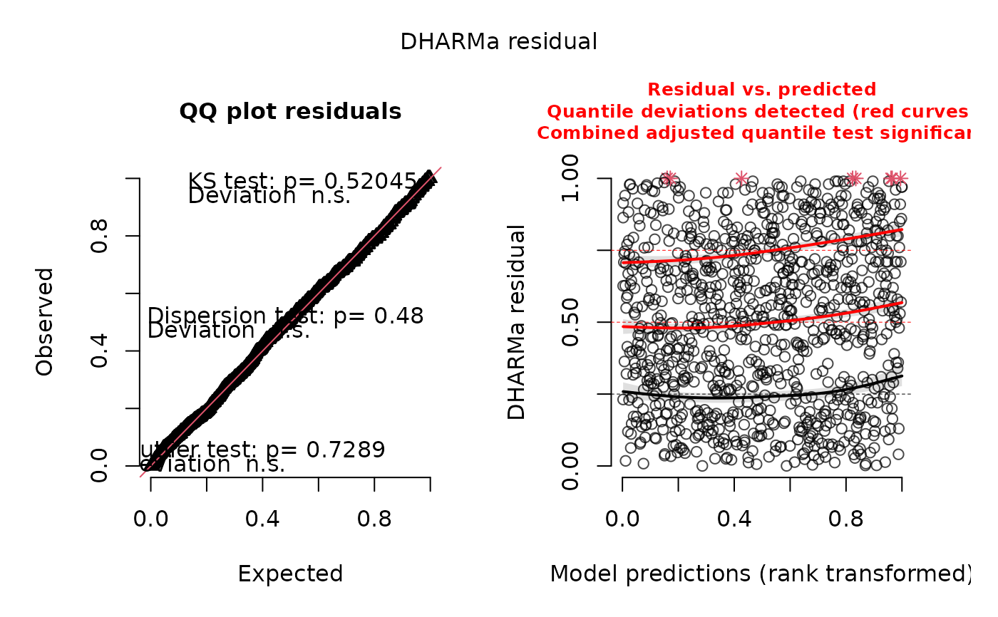
Plot (and possibly return) DHARMa residuals. This is a wrapper function around DHARMa::createDHARMa() to facilitate its use with sdmTMB() models. Note: It is recommended to set type = "mle-mvn" in simulate.sdmTMB() for the resulting residuals to have the expected distribution. This is not the default.

Usage

dharma_residuals(
  simulated_response,
  object,
  plot = TRUE,
  return_DHARMa = FALSE,
  expected_distribution = c("uniform", "normal"),
  ...
)

Arguments

simulated_response

Output from simulate.sdmTMB(). It is recommended to set type = "mle-mvn" in the call to simulate.sdmTMB() for the residuals to have the expected distribution.

object

Output from sdmTMB().

plot

Logical.

return_DHARMa

Logical.

expected_distribution

Experimental: expected distribution for comparison: uniform(0, 1) or normal(0, 1). Traditional DHARMa residuals are uniform. If "normal", a pnorm() transformation is applied. First, any simulated quantiles of 0 (no simulations were smaller than the observation) are set to an arbitrary value of 1/(n*10) where n is the number of simulated replicated. Any simulated quantiles of 1 (no simulations were larger than the observation) are set to an arbitrary value of 1 - 1/(n*10). These points are shown with crosses overlaid.

...

Other arguments to pass to DHARMa::createDHARMa().

Value

A data frame of observed and expected values is invisibly returned, so you can set plot = FALSE and assign the output to an object if you wish to plot the residuals yourself. See the examples.

If return_DHARMa = TRUE, the object from DHARMa::createDHARMa()

is returned and any subsequent DHARMa functions can be applied.

Details

Advantages to these residuals over the ones from the residuals.sdmTMB() method are (1) they work with delta/hurdle models for the combined predictions, not the just the two parts separately, (2) they should work for all families, not the just the families where we have worked out the analytical quantile function, and (3) they can be used with the various diagnostic tools and plots from the DHARMa package.

Disadvantages are (1) they are slower to calculate since one must first simulate from the model, (2) the stability of the distribution of the residuals depends on having a sufficient number of simulation draws, (3) uniformly distributed residuals put less emphasis on the tails visually (which or may not be desired).

Note that DHARMa returns residuals that are uniform(0, 1) if the data are consistent with the model whereas any randomized quantile residuals from residuals.sdmTMB() are expected to be normal(0, 1). An experimental option expected_distribution is included to transform the distributions to a normal(0, 1) expectation.

See also

simulate.sdmTMB(), residuals.sdmTMB()

Examples

# Try Tweedie family:
fit <- sdmTMB(density ~ as.factor(year) + s(depth, k = 3),
  data = pcod_2011, mesh = pcod_mesh_2011,
  family = tweedie(link = "log"), spatial = "on")

# The `simulated_response` argument is first so the output from
# simulate() can be piped to dharma_residuals().

# We will work with 100 simulations for fast examples, but you'll
# likely want to work with more than this (enough that the results
# are stable from run to run).

# not great:
set.seed(123)
simulate(fit, nsim = 100, type = "mle-mvn") |>
  dharma_residuals(fit)


# \donttest{
# delta-lognormal looks better:
set.seed(123)
fit_dl <- update(fit, family = delta_lognormal())
simulate(fit_dl, nsim = 100, type = "mle-mvn") |>
  dharma_residuals(fit)


# or skip the pipe:
set.seed(123)
s <- simulate(fit_dl, nsim = 100, type = "mle-mvn")
# and manually plot it:
r <- dharma_residuals(s, fit_dl, plot = FALSE)
head(r)
#>       observed    expected
#> 1 0.0002512885 0.001030928
#> 2 0.0003998549 0.002061856
#> 3 0.0017916820 0.003092784
#> 4 0.0030243763 0.004123711
#> 5 0.0032777465 0.005154639
#> 6 0.0060709249 0.006185567
plot(r$expected, r$observed)
abline(0, 1)


# return the DHARMa object and work with the DHARMa methods
ret <- simulate(fit_dl, nsim = 100, type = "mle-mvn") |>
  dharma_residuals(fit, return_DHARMa = TRUE)
plot(ret)


# try normal(0, 1) residuals:
s <- simulate(fit_dl, nsim = 100, type = "mle-mvn")
dharma_residuals(s, fit, expected_distribution = "normal")

# note the points in the top right corner that had Inf quantiles
# because of pnorm(1)

# work with the residuals themselves:
r <- dharma_residuals(s, fit, return_DHARMa = TRUE)
plot(fitted(fit), r$scaledResiduals)

# }