Plot anisotropy from an sdmTMB model — plot

Anisotropy is when spatial correlation is directionally dependent. In sdmTMB(), the default spatial correlation is isotropic, but anisotropy can be enabled with anisotropy = TRUE. These plotting functions help visualize that estimated anisotropy.

Usage

plot_anisotropy(object, return_data = FALSE)

plot_anisotropy2(object, model = 1)

Arguments

object: An object from sdmTMB().
return_data: Logical. Return a data frame? plot_anisotropy() only.
model: Which model if a delta model (only for plot_anisotropy2(); plot_anisotropy() always plots both).

Value

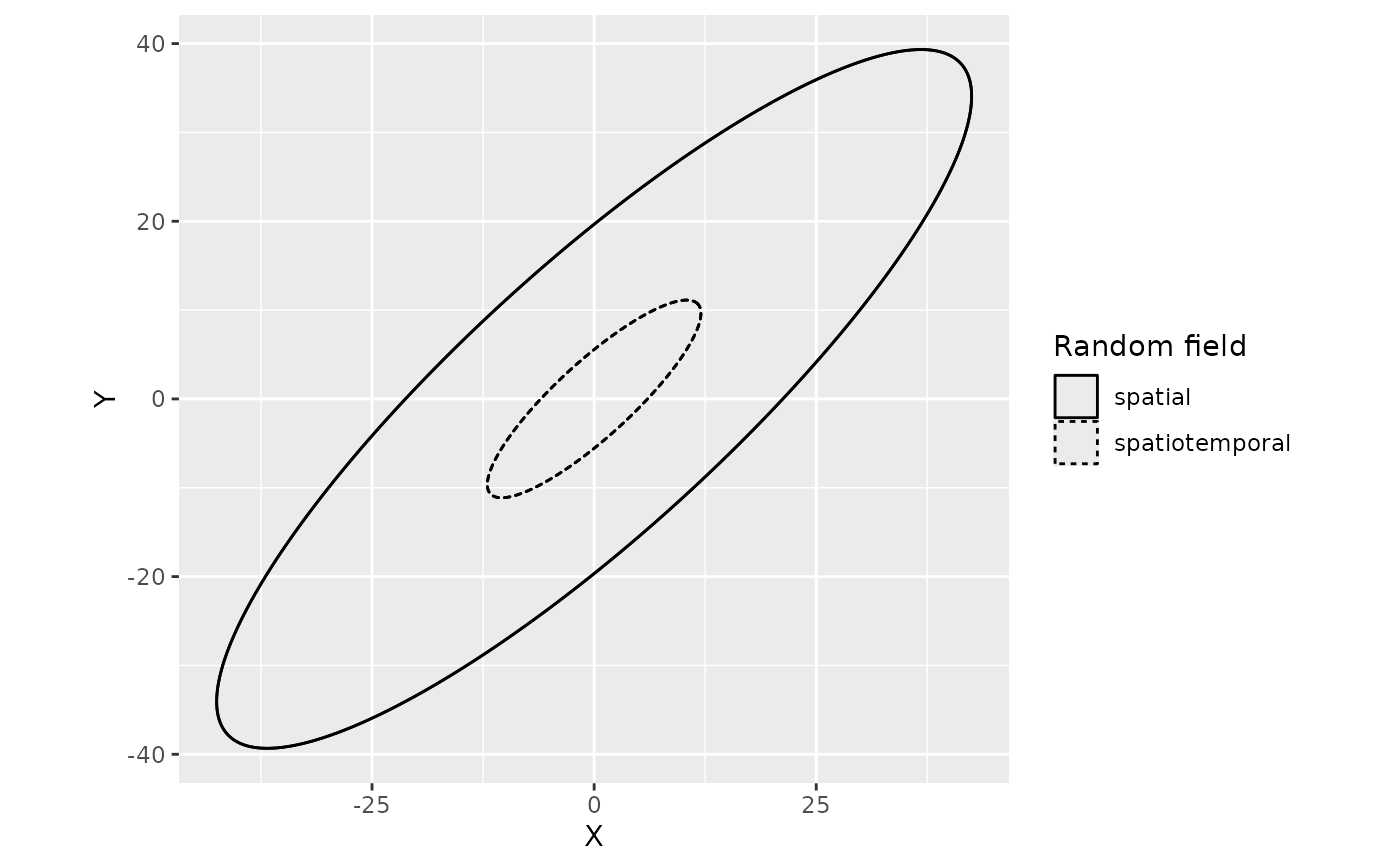
plot_anisotropy(): One or more ellipses illustrating the estimated anisotropy. The ellipses are centered at coordinates of zero in the space of the X-Y coordinates being modeled. The ellipses show the spatial and/or spatiotemporal range (distance at which correlation is effectively independent) in any direction from zero. Uses ggplot2. If anisotropy was turned off when fitting the model, NULL is returned instead of a ggplot2 object.

plot_anisotropy2(): A plot of eigenvectors illustrating the estimated anisotropy. A list of the plotted data is invisibly returned. Uses base graphics. If anisotropy was turned off when fitting the model, NULL is returned instead of a plot object.

References

Code adapted from VAST R package

Examples

mesh <- make_mesh(pcod_2011, c("X", "Y"), n_knots = 80, type = "kmeans")
fit <- sdmTMB(
  data = pcod_2011,
  formula = density ~ 1,
  mesh = mesh,
  family = tweedie(),
  share_range = FALSE,
  time = "year",
  anisotropy = TRUE #<
)
plot_anisotropy(fit)

plot_anisotropy2(fit)