Simulate from a spatial/spatiotemporal model

sdmTMB_simulate() uses TMB to simulate new data given specified parameter values. simulate.sdmTMB(), on the other hand, takes an existing model fit and simulates new observations and optionally new random effects.

Usage

sdmTMB_simulate(
  formula,
  data,
  mesh,
  family = gaussian(link = "identity"),
  time = NULL,
  B = NULL,
  range = NULL,
  rho = NULL,
  sigma_O = NULL,
  sigma_E = NULL,
  sigma_Z = NULL,
  phi = NULL,
  tweedie_p = NULL,
  df = NULL,
  threshold_coefs = NULL,
  fixed_re = list(omega_s = NULL, epsilon_st = NULL, zeta_s = NULL),
  previous_fit = NULL,
  seed = sample.int(1e+06, 1),
  ...
)

Arguments

formula: A one-sided formula describing the fixed-effect structure. Random intercepts are not (yet) supported. Fixed effects should match the corresponding B argument vector of coefficient values.
data: A data frame containing the predictors described in formula and the time column if time is specified.
mesh: Output from make_mesh().
family: Family as in sdmTMB(). Delta families are not supported. Instead, simulate the two component models separately and combine.
time: The time column name.
B: A vector of beta values (fixed-effect coefficient values).
range: Parameter that controls the decay of spatial correlation. If a vector of length 2, share_range will be set to FALSE and the spatial and spatiotemporal ranges will be unique.
rho: Spatiotemporal correlation between years; should be between -1 and 1.
sigma_O: SD of spatial process (Omega).
sigma_E: SD of spatiotemporal process (Epsilon).
sigma_Z: SD of spatially varying coefficient field (Zeta).
phi: Observation error scale parameter (e.g., SD in Gaussian).
tweedie_p: Tweedie p (power) parameter; between 1 and 2.
df: Student-t degrees of freedom.
threshold_coefs: An optional vector of threshold coefficient values if the formula includes breakpt() or logistic(). If breakpt(), these are slope and cut values. If logistic(), these are the threshold at which the function is 50% of the maximum, the threshold at which the function is 95% of the maximum, and the maximum. See the model description vignette for details.
fixed_re: A list of optional random effects to fix at specified (e.g., previously estimated) values. Values of NULL will result in the random effects being simulated.
previous_fit: (Deprecated; please use simulate.sdmTMB()). An optional previous sdmTMB() fit to pull parameter values. Will be over-ruled by any non-NULL specified parameter arguments.
seed: Seed number.
...: Any other arguments to pass to sdmTMB().

Value

A data frame where:

The 1st column is the time variable (if present).
The 2nd and 3rd columns are the spatial coordinates.
omega_s represents the simulated spatial random effects (only if present).
zeta_s represents the simulated spatial varying covariate field (only if present).
epsilon_st represents the simulated spatiotemporal random effects (only if present).
eta is the true value in link space
mu is the true value in inverse link space.
observed represents the simulated process with observation error.
The remaining columns are the fixed-effect model matrix.

Examples

  set.seed(123)

  # make fake predictor(s) (a1) and sampling locations:
  predictor_dat <- data.frame(
    X = runif(300), Y = runif(300),
    a1 = rnorm(300), year = rep(1:6, each = 50)
  )
  mesh <- make_mesh(predictor_dat, xy_cols = c("X", "Y"), cutoff = 0.1)

  sim_dat <- sdmTMB_simulate(
    formula = ~ 1 + a1,
    data = predictor_dat,
    time = "year",
    mesh = mesh,
    family = gaussian(),
    range = 0.5,
    sigma_E = 0.1,
    phi = 0.1,
    sigma_O = 0.2,
    seed = 42,
    B = c(0.2, -0.4) # B0 = intercept, B1 = a1 slope
  )
  head(sim_dat)
#>   year         X           Y     omega_s  epsilon_st         mu        eta
#> 1    1 0.2875775 0.784575267 -0.02131861 -0.02779393  0.4369843  0.4369843
#> 2    1 0.7883051 0.009429905  0.28852319  0.09092583  0.8805246  0.8805246
#> 3    1 0.4089769 0.779065883  0.13541643 -0.08468148  0.6261504  0.6261504
#> 4    1 0.8830174 0.729390652  0.28597232 -0.01660011  0.8903775  0.8903775
#> 5    1 0.9404673 0.630131853  0.21070545  0.02005202  0.6056213  0.6056213
#> 6    1 0.0455565 0.480910830 -0.08071932 -0.11409909 -0.1272901 -0.1272901
#>     observed (Intercept)         a1
#> 1  0.4176273           1 -0.7152422
#> 2  0.8802910           1 -0.7526890
#> 3  0.6248675           1 -0.9385387
#> 4  0.9055722           1 -1.0525133
#> 5  0.6654724           1 -0.4371595
#> 6 -0.1399113           1  0.3311792

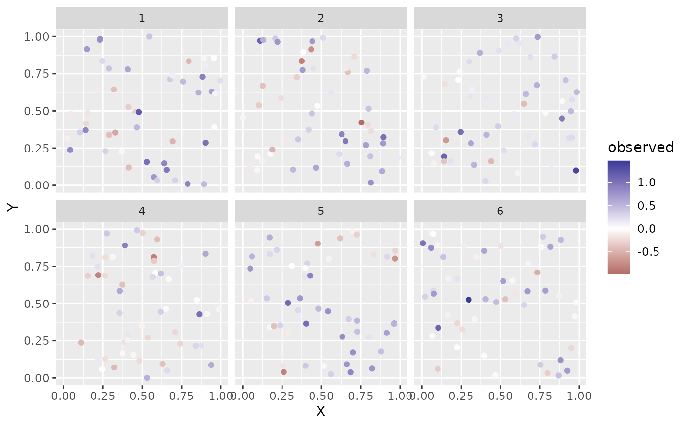
  if (require("ggplot2", quietly = TRUE)) {
    ggplot(sim_dat, aes(X, Y, colour = observed)) +
      geom_point() +
      facet_wrap(~year) +
      scale_color_gradient2()
  }


  # fit to the simulated data:
  fit <- sdmTMB(observed ~ a1, data = sim_dat, mesh = mesh, time = "year")
  fit
#> Spatiotemporal model fit by ML ['sdmTMB']
#> Formula: observed ~ a1
#> Mesh: mesh (isotropic covariance)
#> Time column: year
#> Data: sim_dat
#> Family: gaussian(link = 'identity')
#>  
#>             coef.est coef.se
#> (Intercept)     0.23    0.09
#> a1             -0.39    0.01
#> 
#> Dispersion parameter: 0.09
#> Matérn range: 0.40
#> Spatial SD: 0.21
#> Spatiotemporal IID SD: 0.11
#> ML criterion at convergence: -162.527
#> 
#> See ?tidy.sdmTMB to extract these values as a data frame.

Usage

Arguments

Value

See also

Examples