Area-weighted age composition standardization with sdmTMB

library(sdmTMB)
library(fmesher)
library(ggplot2)
library(dplyr)
theme_set(theme_minimal())

This document shows area-weighted age composition expansion with sdmTMB using simulated data. In other words, we use area-expansion to calculate proportion-at-age using (potentially) spatially unbalanced sampling data. Please see Thorson and Haltuch (2018) for further description.

We will start by simulating some data. This simulation code chunk is hidden for simplicity.

We can look at the simulated data:

head(data)
#>   year         x          y abundance_per_area   age   year_age
#> 1 2018 0.2875775 0.63918581         0.51004952 age_1 2018_age_1
#> 2 2018 0.7883051 0.12482240         1.60038328 age_1 2018_age_1
#> 3 2018 0.4089769 0.25526578         0.00000000 age_1 2018_age_1
#> 4 2018 0.8830174 0.82057469         0.04387091 age_1 2018_age_1
#> 5 2018 0.9404673 0.80378039         1.27301974 age_1 2018_age_1
#> 6 2018 0.0455565 0.04583463         0.86470310 age_1 2018_age_1

We are assuming that the these data have already gone “first stage expansion”. I.e., each subsample has been expanded to represent the total abundance (or biomass) of the primary sample from which it came. Although we model abundance per area here, we could alternatively model abundance with an offset for (log) area.

Plot the raw simulated data:

ggplot(data, aes(x, y, colour = log(abundance_per_area + 1))) +
  geom_point() +
  facet_grid(year ~ age) +
  scale_colour_viridis_c() +
  labs(colour = "Abundance\nper\narea")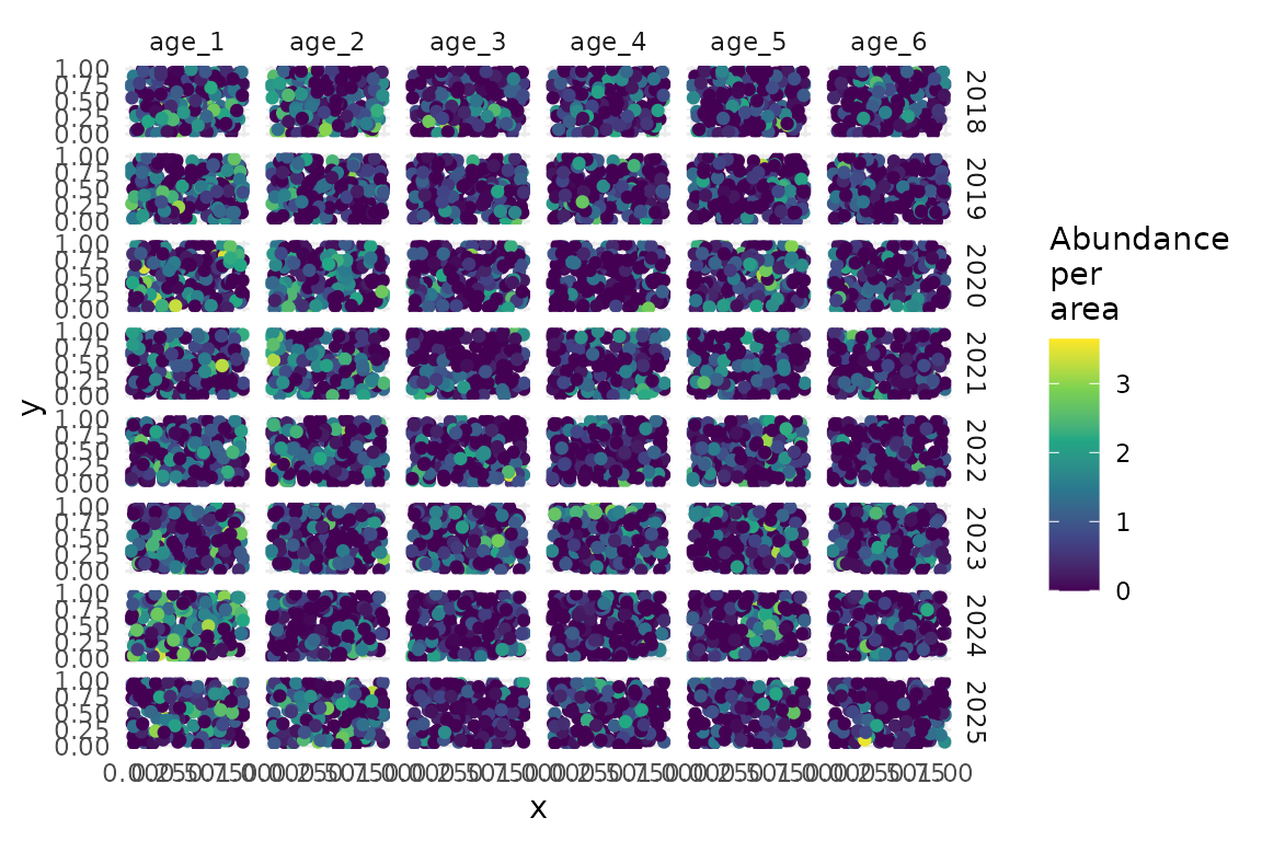


# Show data for one year
data_subset <- filter(data, year == 2021)
ggplot(data_subset, aes(x, y, size = abundance_per_area, colour = age)) +
  geom_point(alpha = 0.7) +
  facet_wrap(~age) +
  labs(title = "Simulated data (2021)", size = "Abundance per area")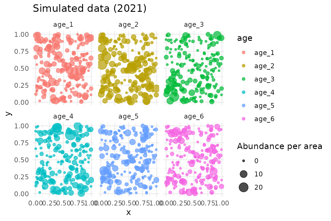

Now we will set up the spatial and spatiotemporal fields with shared SDs across ages. This could alternatively be set up to have different spatial SDs by age and/or different spatiotemporal SDs by age.

mesh_sdm <- make_mesh(data, c("x", "y"), cutoff = 0.1)

# Use a helper function to set up the model components
svc_setup <- sdmTMB::setup_category_svc(
  data = data,
  category_column = "age",
  time_column = "year",
  share_spatial_sd = TRUE, # All ages share spatial SD
  share_spatiotemporal_sd = TRUE # All age-year combinations share spatiotemporal SD
)

This would return information on what just ran:

svc_setup$info

The important parts are the following.

Our data frame has additional columns for use in the spatial_varying argument:

colnames(svc_setup$data_expanded)
#>  [1] "year"                      "x"                        
#>  [3] "y"                         "abundance_per_area"       
#>  [5] "age"                       "year_age"                 
#>  [7] "ageage_1"                  "ageage_2"                 
#>  [9] "ageage_3"                  "ageage_4"                 
#> [11] "ageage_5"                  "ageage_6"                 
#> [13] "factor(year)2018:ageage_1" "factor(year)2019:ageage_1"
#> [15] "factor(year)2020:ageage_1" "factor(year)2021:ageage_1"
#> [17] "factor(year)2022:ageage_1" "factor(year)2023:ageage_1"
#> [19] "factor(year)2024:ageage_1" "factor(year)2025:ageage_1"
#> [21] "factor(year)2018:ageage_2" "factor(year)2019:ageage_2"
#> [23] "factor(year)2020:ageage_2" "factor(year)2021:ageage_2"
#> [25] "factor(year)2022:ageage_2" "factor(year)2023:ageage_2"
#> [27] "factor(year)2024:ageage_2" "factor(year)2025:ageage_2"
#> [29] "factor(year)2018:ageage_3" "factor(year)2019:ageage_3"
#> [31] "factor(year)2020:ageage_3" "factor(year)2021:ageage_3"
#> [33] "factor(year)2022:ageage_3" "factor(year)2023:ageage_3"
#> [35] "factor(year)2024:ageage_3" "factor(year)2025:ageage_3"
#> [37] "factor(year)2018:ageage_4" "factor(year)2019:ageage_4"
#> [39] "factor(year)2020:ageage_4" "factor(year)2021:ageage_4"
#> [41] "factor(year)2022:ageage_4" "factor(year)2023:ageage_4"
#> [43] "factor(year)2024:ageage_4" "factor(year)2025:ageage_4"
#> [45] "factor(year)2018:ageage_5" "factor(year)2019:ageage_5"
#> [47] "factor(year)2020:ageage_5" "factor(year)2021:ageage_5"
#> [49] "factor(year)2022:ageage_5" "factor(year)2023:ageage_5"
#> [51] "factor(year)2024:ageage_5" "factor(year)2025:ageage_5"
#> [53] "factor(year)2018:ageage_6" "factor(year)2019:ageage_6"
#> [55] "factor(year)2020:ageage_6" "factor(year)2021:ageage_6"
#> [57] "factor(year)2022:ageage_6" "factor(year)2023:ageage_6"
#> [59] "factor(year)2024:ageage_6" "factor(year)2025:ageage_6"

We have a formula for the spatial_varying argument:

svc_setup$svc_formula
#> ~ageage_1 + ageage_2 + ageage_3 + ageage_4 + ageage_5 + ageage_6 + 
#>     `factor(year)2018:ageage_1` + `factor(year)2019:ageage_1` + 
#>     `factor(year)2020:ageage_1` + `factor(year)2021:ageage_1` + 
#>     `factor(year)2022:ageage_1` + `factor(year)2023:ageage_1` + 
#>     `factor(year)2024:ageage_1` + `factor(year)2025:ageage_1` + 
#>     `factor(year)2018:ageage_2` + `factor(year)2019:ageage_2` + 
#>     `factor(year)2020:ageage_2` + `factor(year)2021:ageage_2` + 
#>     `factor(year)2022:ageage_2` + `factor(year)2023:ageage_2` + 
#>     `factor(year)2024:ageage_2` + `factor(year)2025:ageage_2` + 
#>     `factor(year)2018:ageage_3` + `factor(year)2019:ageage_3` + 
#>     `factor(year)2020:ageage_3` + `factor(year)2021:ageage_3` + 
#>     `factor(year)2022:ageage_3` + `factor(year)2023:ageage_3` + 
#>     `factor(year)2024:ageage_3` + `factor(year)2025:ageage_3` + 
#>     `factor(year)2018:ageage_4` + `factor(year)2019:ageage_4` + 
#>     `factor(year)2020:ageage_4` + `factor(year)2021:ageage_4` + 
#>     `factor(year)2022:ageage_4` + `factor(year)2023:ageage_4` + 
#>     `factor(year)2024:ageage_4` + `factor(year)2025:ageage_4` + 
#>     `factor(year)2018:ageage_5` + `factor(year)2019:ageage_5` + 
#>     `factor(year)2020:ageage_5` + `factor(year)2021:ageage_5` + 
#>     `factor(year)2022:ageage_5` + `factor(year)2023:ageage_5` + 
#>     `factor(year)2024:ageage_5` + `factor(year)2025:ageage_5` + 
#>     `factor(year)2018:ageage_6` + `factor(year)2019:ageage_6` + 
#>     `factor(year)2020:ageage_6` + `factor(year)2021:ageage_6` + 
#>     `factor(year)2022:ageage_6` + `factor(year)2023:ageage_6` + 
#>     `factor(year)2024:ageage_6` + `factor(year)2025:ageage_6`
#> <environment: 0x561542dc5b08>

And we have a TMB ‘map’ list, which controls which random field SDs are shared vs. estimated separately. Factor levels that are the same get shared; those that are different are estimated separately.

svc_setup$svc_map
#> $ln_tau_Z
#>  [1] 1 1 1 1 1 1 2 2 2 2 2 2 2 2 2 2 2 2 2 2 2 2 2 2 2 2 2 2 2 2 2 2 2 2 2 2 2 2
#> [39] 2 2 2 2 2 2 2 2 2 2 2 2 2 2 2 2
#> Levels: 1 2

Internally, ln_tau_Z is a precision parameter that affects the SD of the SVC fields.

We’ll set up a control list. The only critical part is the map argument.

control_sdmTMB <- sdmTMBcontrol(
  map = svc_setup$svc_map, # critical part
  multiphase = FALSE, # often faster here
  newton_loops = 0, # for a faster example
  profile = "b_j", # often faster here
  getsd = TRUE # skip running sdreport() if desired for speed while testing
)

Fit our model:

fit_sdmTMB <- sdmTMB(
  abundance_per_area ~ 0 + year_age,
  mesh = mesh_sdm,
  data = svc_setup$data_expanded, # Use expanded data
  family = tweedie(),
  time = "year",
  spatial = "off", # all spatial variation with spatial_varying
  spatiotemporal = "off", # all spatiotemporal variation with spatial_varying
  spatial_varying = svc_setup$svc_formula,
  silent = FALSE,
  control = control_sdmTMB
)
#> ℹ Fixing or mirroring `ln_tau_Z`
#> running TMB sdreport

sanity(fit_sdmTMB)
#> ✔ Non-linear minimizer suggests successful convergence
#> ✔ Hessian matrix is positive definite
#> ✔ No extreme or very small eigenvalues detected
#> ✔ No gradients with respect to fixed effects are >= 0.001
#> ✔ No fixed-effect standard errors are NA
#> ✔ No standard errors look unreasonably large
#> ✔ No sigma parameters are < 0.01
#> ✔ No sigma parameters are > 100
#> ✔ Range parameter doesn't look unreasonably large
fit_sdmTMB
#> Spatial model fit by ML ['sdmTMB']
#> Formula: abundance_per_area ~ 0 + year_age
#> Mesh: mesh_sdm (isotropic covariance)
#> Time column: year
#> Data: svc_setup$data_expanded
#> Family: tweedie(link = 'log')
#>  
#> Conditional model:
#>                    coef.est coef.se
#> year_age2018_age_1     0.73    0.19
#> year_age2018_age_2     0.81    0.19
#> year_age2018_age_3    -0.08    0.20
#> year_age2018_age_4     0.00    0.20
#> year_age2018_age_5     0.24    0.20
#> year_age2018_age_6     0.11    0.20
#> year_age2019_age_1     0.78    0.19
#> year_age2019_age_2     0.41    0.19
#> year_age2019_age_3     0.13    0.20
#> year_age2019_age_4    -0.01    0.20
#> year_age2019_age_5     0.13    0.20
#> year_age2019_age_6    -0.28    0.20
#> year_age2020_age_1     0.79    0.19
#> year_age2020_age_2     0.80    0.19
#> year_age2020_age_3     0.13    0.20
#> year_age2020_age_4    -0.39    0.21
#> year_age2020_age_5     0.66    0.19
#> year_age2020_age_6     0.27    0.20
#> year_age2021_age_1     0.51    0.19
#> year_age2021_age_2     0.88    0.19
#> year_age2021_age_3    -0.17    0.20
#> year_age2021_age_4     0.29    0.20
#> year_age2021_age_5     0.10    0.20
#> year_age2021_age_6    -0.08    0.20
#> year_age2022_age_1     0.39    0.19
#> year_age2022_age_2     0.68    0.19
#> year_age2022_age_3     0.26    0.20
#> year_age2022_age_4    -0.03    0.20
#> year_age2022_age_5     0.50    0.19
#> year_age2022_age_6    -0.47    0.21
#> year_age2023_age_1     0.69    0.19
#> year_age2023_age_2     0.55    0.19
#> year_age2023_age_3     0.40    0.19
#> year_age2023_age_4     0.40    0.19
#> year_age2023_age_5     0.22    0.20
#> year_age2023_age_6     0.12    0.20
#> year_age2024_age_1     1.32    0.18
#> year_age2024_age_2     0.19    0.20
#> year_age2024_age_3     0.06    0.20
#> year_age2024_age_4    -0.31    0.20
#> year_age2024_age_5     0.09    0.20
#> year_age2024_age_6    -0.18    0.20
#> year_age2025_age_1     0.58    0.19
#> year_age2025_age_2     0.82    0.19
#> year_age2025_age_3    -0.39    0.21
#> year_age2025_age_4    -0.01    0.20
#> year_age2025_age_5     0.12    0.20
#> year_age2025_age_6    -0.26    0.20
#> 
#> Dispersion parameter: 2.99
#> Tweedie p: 1.60
#> Matérn range: 0.20
#> Spatially varying coefficient SD (ageage_1): 0.47
#> Spatially varying coefficient SD (ageage_2): 0.47
#> Spatially varying coefficient SD (ageage_3): 0.47
#> Spatially varying coefficient SD (ageage_4): 0.47
#> Spatially varying coefficient SD (ageage_5): 0.47
#> Spatially varying coefficient SD (ageage_6): 0.47
#> Spatially varying coefficient SD (`factor(year)2018:ageage_1`): 0.51
#> Spatially varying coefficient SD (`factor(year)2019:ageage_1`): 0.51
#> Spatially varying coefficient SD (`factor(year)2020:ageage_1`): 0.51
#> Spatially varying coefficient SD (`factor(year)2021:ageage_1`): 0.51
#> Spatially varying coefficient SD (`factor(year)2022:ageage_1`): 0.51
#> Spatially varying coefficient SD (`factor(year)2023:ageage_1`): 0.51
#> Spatially varying coefficient SD (`factor(year)2024:ageage_1`): 0.51
#> Spatially varying coefficient SD (`factor(year)2025:ageage_1`): 0.51
#> Spatially varying coefficient SD (`factor(year)2018:ageage_2`): 0.51
#> Spatially varying coefficient SD (`factor(year)2019:ageage_2`): 0.51
#> Spatially varying coefficient SD (`factor(year)2020:ageage_2`): 0.51
#> Spatially varying coefficient SD (`factor(year)2021:ageage_2`): 0.51
#> Spatially varying coefficient SD (`factor(year)2022:ageage_2`): 0.51
#> Spatially varying coefficient SD (`factor(year)2023:ageage_2`): 0.51
#> Spatially varying coefficient SD (`factor(year)2024:ageage_2`): 0.51
#> Spatially varying coefficient SD (`factor(year)2025:ageage_2`): 0.51
#> Spatially varying coefficient SD (`factor(year)2018:ageage_3`): 0.51
#> Spatially varying coefficient SD (`factor(year)2019:ageage_3`): 0.51
#> Spatially varying coefficient SD (`factor(year)2020:ageage_3`): 0.51
#> Spatially varying coefficient SD (`factor(year)2021:ageage_3`): 0.51
#> Spatially varying coefficient SD (`factor(year)2022:ageage_3`): 0.51
#> Spatially varying coefficient SD (`factor(year)2023:ageage_3`): 0.51
#> Spatially varying coefficient SD (`factor(year)2024:ageage_3`): 0.51
#> Spatially varying coefficient SD (`factor(year)2025:ageage_3`): 0.51
#> Spatially varying coefficient SD (`factor(year)2018:ageage_4`): 0.51
#> Spatially varying coefficient SD (`factor(year)2019:ageage_4`): 0.51
#> Spatially varying coefficient SD (`factor(year)2020:ageage_4`): 0.51
#> Spatially varying coefficient SD (`factor(year)2021:ageage_4`): 0.51
#> Spatially varying coefficient SD (`factor(year)2022:ageage_4`): 0.51
#> Spatially varying coefficient SD (`factor(year)2023:ageage_4`): 0.51
#> Spatially varying coefficient SD (`factor(year)2024:ageage_4`): 0.51
#> Spatially varying coefficient SD (`factor(year)2025:ageage_4`): 0.51
#> Spatially varying coefficient SD (`factor(year)2018:ageage_5`): 0.51
#> Spatially varying coefficient SD (`factor(year)2019:ageage_5`): 0.51
#> Spatially varying coefficient SD (`factor(year)2020:ageage_5`): 0.51
#> Spatially varying coefficient SD (`factor(year)2021:ageage_5`): 0.51
#> Spatially varying coefficient SD (`factor(year)2022:ageage_5`): 0.51
#> Spatially varying coefficient SD (`factor(year)2023:ageage_5`): 0.51
#> Spatially varying coefficient SD (`factor(year)2024:ageage_5`): 0.51
#> Spatially varying coefficient SD (`factor(year)2025:ageage_5`): 0.51
#> Spatially varying coefficient SD (`factor(year)2018:ageage_6`): 0.51
#> Spatially varying coefficient SD (`factor(year)2019:ageage_6`): 0.51
#> Spatially varying coefficient SD (`factor(year)2020:ageage_6`): 0.51
#> Spatially varying coefficient SD (`factor(year)2021:ageage_6`): 0.51
#> Spatially varying coefficient SD (`factor(year)2022:ageage_6`): 0.51
#> Spatially varying coefficient SD (`factor(year)2023:ageage_6`): 0.51
#> Spatially varying coefficient SD (`factor(year)2024:ageage_6`): 0.51
#> Spatially varying coefficient SD (`factor(year)2025:ageage_6`): 0.51
#> ML criterion at convergence: 17325.664
#> 
#> See ?tidy.sdmTMB to extract these values as a data frame.

Area expansion

Now let’s calculate area-weighted abundance indices for each age class. First, we need to set up our ‘grid’ data frame over which we will predict. Here we make a simple grid over our 0-1 simulated survey domain.

# Create prediction grid on the same 0-1 spatial domain
n_pred <- 10
pred_grid <- expand.grid(
  x = seq(0, 1, length.out = n_pred),
  y = seq(0, 1, length.out = n_pred)
)

# Each grid cell area (since we're on 0-1 domain)
cell_area <- (1 / n_pred)^2

# Replicate over years and ages
nd <- replicate_df(pred_grid, "year", years)
nd <- replicate_df(nd, "age", ages)
nd$year_age <- paste(nd$year, nd$age, sep = "_")

# Use helper function to add model matrix columns
nd_setup <- sdmTMB::setup_category_svc(
  data = nd,
  category_column = "age",
  time_column = "year",
  share_spatial_sd = TRUE,
  share_spatiotemporal_sd = TRUE
)

Calculate indices for each age:

ind_list <- lapply(ages, function(age) {
  cat("Calculating index for age:", age, "\n")

  # Subset prediction data for this age
  nd_age <- nd_setup$data_expanded[nd_setup$data_expanded$age == age, ]

  # Get predictions
  pred <- predict(fit_sdmTMB, newdata = nd_age, return_tmb_object = TRUE)

  # Calculate area-weighted index
  ind <- get_index(pred, area = cell_area, bias_correct = TRUE)
  data.frame(ind, age = age)
})

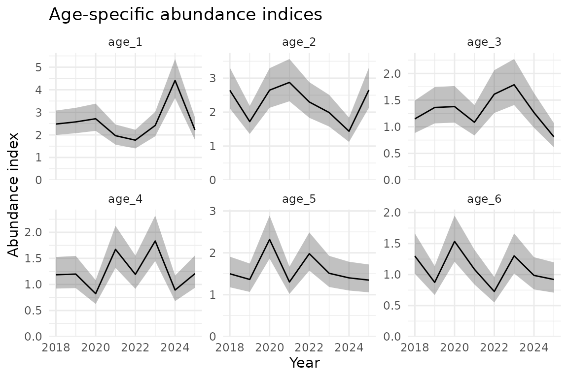
ind <- do.call(rbind, ind_list)

Plot abundance indices by age:

ggplot(ind, aes(year, est)) +
  geom_ribbon(aes(ymin = lwr, ymax = upr), alpha = 0.3) +
  geom_line() +
  facet_wrap(~age, scales = "free_y") +
  scale_y_continuous(limits = c(0, NA), expand = expansion(mult = c(0, 0.05))) +
  labs(
    x = "Year",
    y = "Abundance index",
    title = "Age-specific abundance indices"
  )

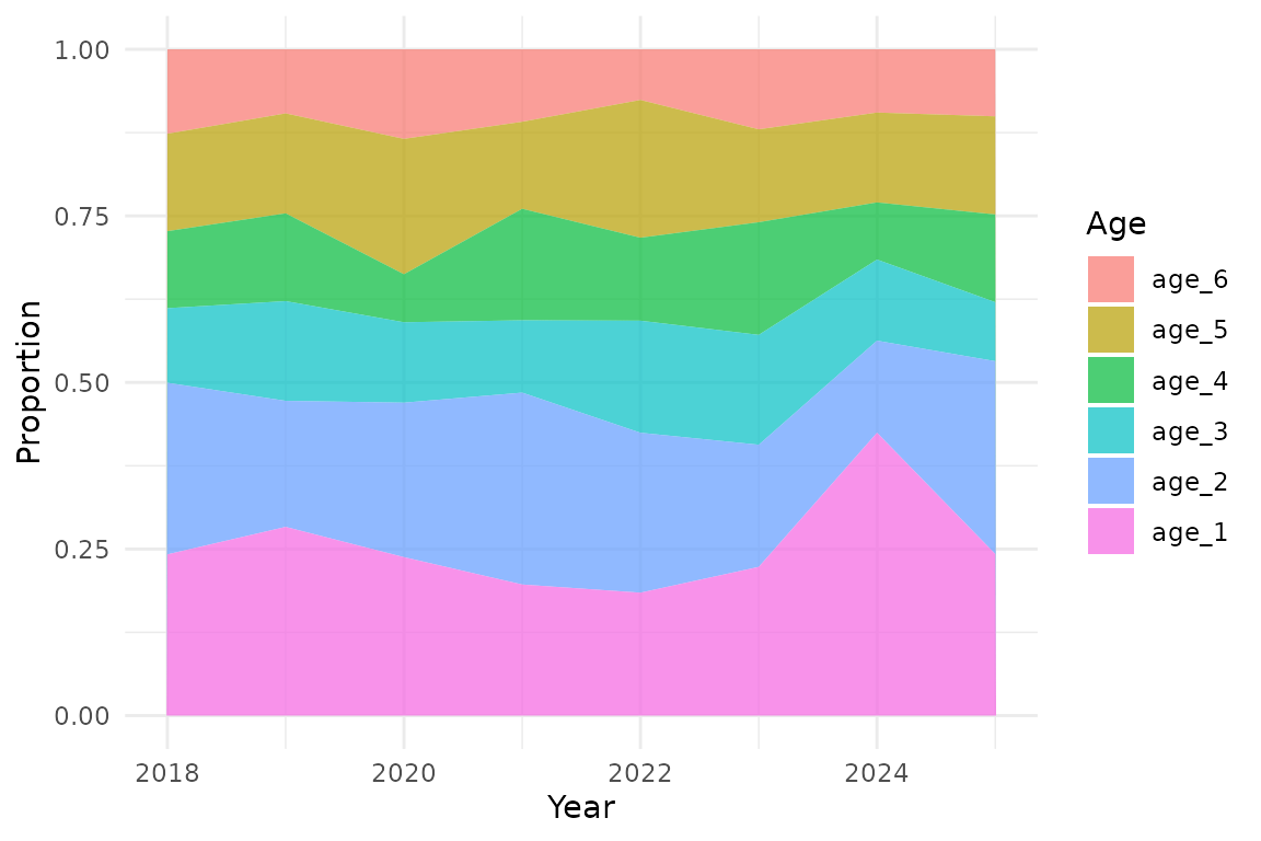
Convert to age composition (proportions)

Convert the abundance indices to proportions-at-age:

ind_props <- ind |>
  group_by(year) |>
  mutate(
    total = sum(est),
    proportion = est / total
  ) |>
  ungroup()

Plot age composition:

ggplot(ind_props, aes(year, proportion, fill = factor(age, levels = rev(ages)))) +
  geom_area(position = "stack", alpha = 0.7) +
  labs(
    x = "Year",
    y = "Proportion",
    fill = "Age",
  )


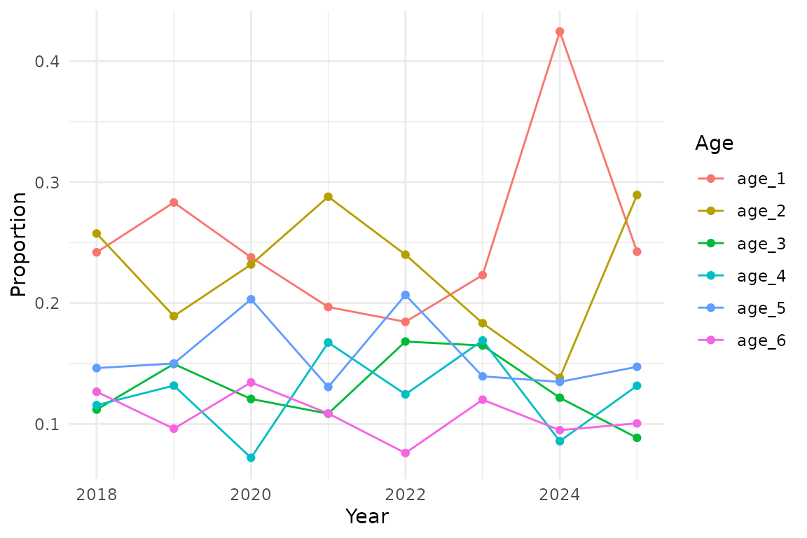
ggplot(ind_props, aes(year, proportion, colour = age)) +
  geom_line() +
  geom_point() +
  labs(
    x = "Year",
    y = "Proportion",
    colour = "Age",
  )

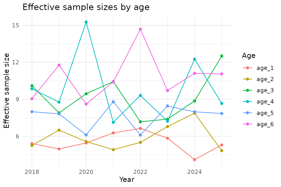
Calculate effective sample sizes

Here we’ll calculate effective sample sizes for the age composition, following the method from VAST (Thorson 2019) as described in Thorson and Haltuch (2018).

# Function to calculate effective sample sizes from index estimates
# This may be folded into sdmTMB eventually
get_comp_neff <- function(dat, index_df, time_column = "year", bin_column = "age") {
  # Get unique years and ages in original order
  years_unique <- unique(dat[[time_column]])
  bins_unique <- unique(dat[[bin_column]])
  nyrs <- length(years_unique)
  nbins <- length(bins_unique)

  # Reshape estimates and SEs to matrices (bins x years)
  est_mat <- t(matrix(index_df$est, nrow = nyrs, ncol = nbins))
  se_mat <- t(matrix(index_df$se_natural, nrow = nyrs, ncol = nbins))

  # Calculate total abundance and SE by year
  total_by_year <- colSums(est_mat)
  total_se_by_year <- sqrt(colSums(se_mat^2))

  # Calculate proportions
  prop_mat <- est_mat / rep(total_by_year, each = nbins)

  # Calculate proportion variance and effective sample sizes using delta method
  var_prop_mat <- matrix(NA, nrow = nbins, ncol = nyrs)
  neff_mat <- matrix(NA, nrow = nbins, ncol = nyrs)

  for (i in 1:nbins) {
    for (j in 1:nyrs) {
      if (est_mat[i, j] > 0) {
        var_prop_mat[i, j] <- est_mat[i, j]^2 / total_by_year[j]^2 *
          (se_mat[i, j]^2 / est_mat[i, j]^2 -
            2 * se_mat[i, j]^2 / (est_mat[i, j] * total_by_year[j]) +
            total_se_by_year[j]^2 / total_by_year[j]^2)
        neff_mat[i, j] <- prop_mat[i, j] * (1 - prop_mat[i, j]) / var_prop_mat[i, j]
      } else {
        var_prop_mat[i, j] <- 0
        neff_mat[i, j] <- 0
      }
    }
  }

  # Calculate median Neff by year
  neff_median <- apply(neff_mat, 2, median, na.rm = TRUE)

  # Convert to data frame
  bin_indices <- rep(1:nbins, nyrs)
  year_indices <- rep(1:nyrs, each = nbins)
  result <- data.frame(
    prop_se = sqrt(as.vector(var_prop_mat)),
    prop = as.vector(prop_mat),
    neff = as.vector(neff_mat),
    neff_median = rep(neff_median, each = nbins)
  )

  # Add year and bin columns
  result[[time_column]] <- years_unique[year_indices]
  result[[bin_column]] <- bins_unique[bin_indices]
  result
}

# Calculate effective sample sizes
neff_results <- get_comp_neff(data, ind)

# Show results
head(neff_results)
#>      prop_se      prop      neff neff_median year   age
#> 1 0.18427485 0.2419754  5.401600    8.519126 2018 age_1
#> 2 0.19090118 0.2575352  5.246810    8.519126 2018 age_2
#> 3 0.09922406 0.1119492 10.097755    8.519126 2018 age_3
#> 4 0.10186871 0.1156016  9.852132    8.519126 2018 age_4
#> 5 0.12500528 0.1462638  7.991050    8.519126 2018 age_5
#> 6 0.11057981 0.1266747  9.047203    8.519126 2018 age_6

Plot effective sample sizes:

ggplot(neff_results, aes(year, neff, colour = age)) +
  geom_line() +
  geom_point() +
  labs(
    x = "Year",
    y = "Effective sample size",
    colour = "Age",
    title = "Effective sample sizes by age"
  )


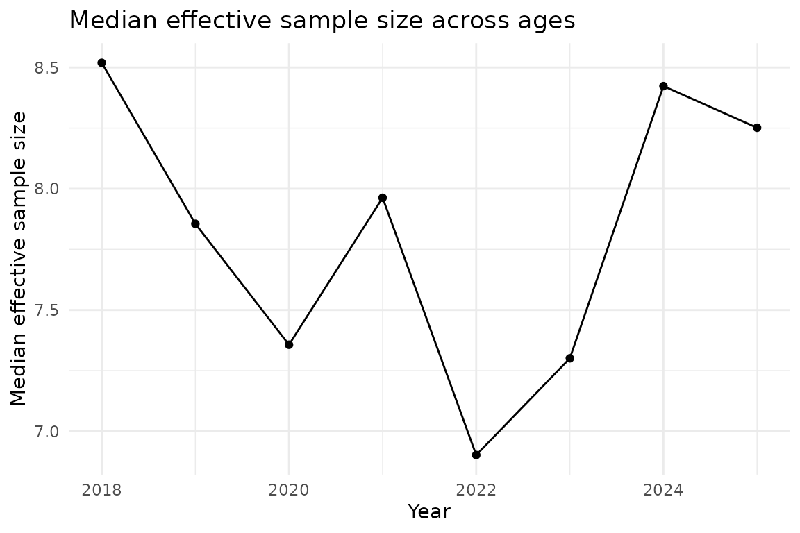
# Plot median effective sample size across ages
neff_median <- neff_results |>
  select(year, neff_median) |>
  distinct()

ggplot(neff_median, aes(year, neff_median)) +
  geom_line() +
  geom_point() +
  labs(
    x = "Year",
    y = "Median effective sample size",
    title = "Median effective sample size across ages"
  )

References

Thorson, J.T., and Haltuch, M.A. 2018. Spatio-temporal analysis of compositional data: increased precision and improved workflow using model-based inputs to stock assessment. Can. J. Fish. Aquat. Sci. doi:10.1139/cjfas-2018-0015.

Thorson, J.T. 2019. Guidance for decisions using the Vector Autoregressive Spatio-Temporal (VAST) package in stock, ecosystem, habitat and climate assessments. Fisheries Research 210: 143–161. doi:10.1016/j.fishres.2018.10.013.

2025-09-04

Area expansion

Convert to age composition (proportions)

Calculate effective sample sizes

References