Make predictions from an sdmTMB model; can predict on the original or new data.
Usage
# S3 method for class 'sdmTMB'
predict(
  object,
  newdata = NULL,
  type = c("link", "response"),
  se_fit = FALSE,
  re_form = NULL,
  re_form_iid = NULL,
  nsim = 0,
  sims_var = "est",
  model = c(NA, 1, 2),
  offset = NULL,
  mcmc_samples = NULL,
  return_tmb_object = FALSE,
  return_tmb_report = FALSE,
  return_tmb_data = FALSE,
  tmbstan_model = deprecated(),
  sims = deprecated(),
  area = deprecated(),
  ...
)
Arguments
- object
A model fitted with
sdmTMB().- newdata
A data frame to make predictions on. This should be a data frame with the same predictor columns as in the fitted data and a time column (if this is a spatiotemporal model) with the same name as in the fitted data.
- type
Should the
estcolumn be in link (default) or response space?- se_fit
Should standard errors on predictions at the new locations given by
newdatabe calculated? Warning: the current implementation can be slow for large data sets or high-resolution projections unlessre_form = NA(omitting random fields). A faster option to approximate point-wise uncertainty is to use thensimargument.- re_form
NULLto specify including all spatial/spatiotemporal random effects in predictions.~0orNAfor population-level predictions. Likely to be used in conjunction withse_fit = TRUE. This does not affectget_index()calculations.- re_form_iid
NULLto specify including all random intercepts in the predictions.~0orNAfor population-level predictions. No other options (e.g., some but not all random intercepts) are implemented yet. Only affects predictions withnewdata. This does affectsget_index().- nsim
If
> 0, simulate from the joint precision matrix withnsimdraws. Returns a matrix ofnrow(data)bynsimrepresenting the estimates of the linear predictor (i.e., in link space). Can be useful for deriving uncertainty on predictions (e.g.,apply(x, 1, sd)) or propagating uncertainty. This is currently the fastest way to characterize uncertainty on predictions in space with sdmTMB.- sims_var
Experimental: Which TMB reported variable from the model should be extracted from the joint precision matrix simulation draws? Defaults to link-space predictions. Options include:
"omega_s","zeta_s","epsilon_st", and"est_rf"(as described below). Other options will be passed verbatim.- model
Type of prediction if a delta/hurdle model and
nsim > 0ormcmc_samplesis supplied:NAreturns the combined prediction from both components on the link scale for the positive component;1or2return the first or second model component only on the link or response scale depending on the argumenttype. For regular prediction from delta models, both sets of predictions are returned.- offset
A numeric vector of optional offset values. If left at default
NULL, the offset is implicitly left at 0.- mcmc_samples
See
extract_mcmc()in the sdmTMBextra package for more details and the Bayesian vignette. If specified, the predict function will return a matrix of a similar form as ifnsim > 0but representing Bayesian posterior samples from the Stan model.- return_tmb_object
Logical. If
TRUE, will include the TMB object in a list format output. Necessary for theget_index()orget_cog()functions.- return_tmb_report
Logical: return the output from the TMB report? For regular prediction, this is all the reported variables at the MLE parameter values. For
nsim > 0or whenmcmc_samplesis supplied, this is a list where each element is a sample and the contents of each element is the output of the report for that sample.- return_tmb_data
Logical: return formatted data for TMB? Used internally.
- tmbstan_model
Deprecated. See
mcmc_samples.- sims
Deprecated. Please use
nsiminstead.- area
Deprecated. Please use
areainget_index().- ...
Not implemented.
Value
If return_tmb_object = FALSE (and nsim = 0 and mcmc_samples = NULL):
A data frame:
est: Estimate in link space (everything is in link space)est_non_rf: Estimate from everything that isn't a random fieldest_rf: Estimate from all random fields combinedomega_s: Spatial (intercept) random field that is constant through timezeta_s: Spatial slope random fieldepsilon_st: Spatiotemporal (intercept) random fields, could be off (zero), IID, AR1, or random walk
If return_tmb_object = TRUE (and nsim = 0 and mcmc_samples = NULL):
A list:
data: The data frame described abovereport: The TMB report on parameter valuesobj: The TMB object returned from the prediction runfit_obj: The original TMB model object
In this case, you likely only need the data element as an end user.
The other elements are included for other functions.
If nsim > 0 or mcmc_samples is not NULL:
A matrix:
Columns represent samples
Rows represent predictions with one row per row of
newdata
Examples
d <- pcod_2011
mesh <- make_mesh(d, c("X", "Y"), cutoff = 30) # a coarse mesh for example speed
m <- sdmTMB(
data = d, formula = density ~ 0 + as.factor(year) + depth_scaled + depth_scaled2,
time = "year", mesh = mesh, family = tweedie(link = "log")
)
# Predictions at original data locations -------------------------------
predictions <- predict(m)
head(predictions)
#> # A tibble: 6 × 17
#> year X Y depth density present lat lon depth_mean depth_sd
#> <int> <dbl> <dbl> <dbl> <dbl> <dbl> <dbl> <dbl> <dbl> <dbl>
#> 1 2011 435. 5718. 241 245. 1 51.6 -130. 5.16 0.445
#> 2 2011 487. 5719. 52 0 0 51.6 -129. 5.16 0.445
#> 3 2011 490. 5717. 47 0 0 51.6 -129. 5.16 0.445
#> 4 2011 545. 5717. 157 0 0 51.6 -128. 5.16 0.445
#> 5 2011 404. 5720. 398 0 0 51.6 -130. 5.16 0.445
#> 6 2011 420. 5721. 486 0 0 51.6 -130. 5.16 0.445
#> # ℹ 7 more variables: depth_scaled <dbl>, depth_scaled2 <dbl>, est <dbl>,
#> # est_non_rf <dbl>, est_rf <dbl>, omega_s <dbl>, epsilon_st <dbl>
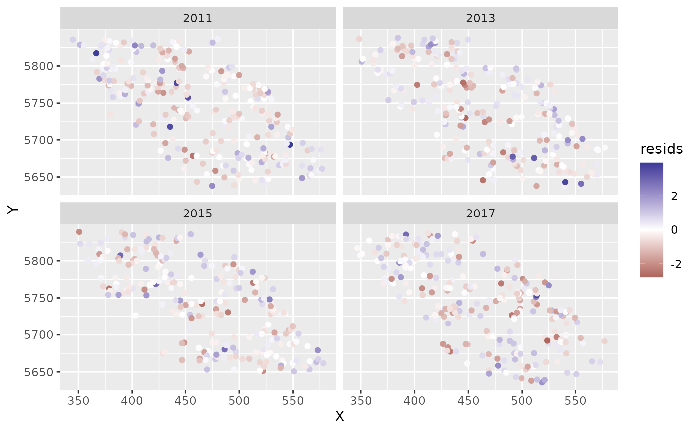
predictions$resids <- residuals(m) # randomized quantile residuals
library(ggplot2)
ggplot(predictions, aes(X, Y, col = resids)) + scale_colour_gradient2() +
geom_point() + facet_wrap(~year)
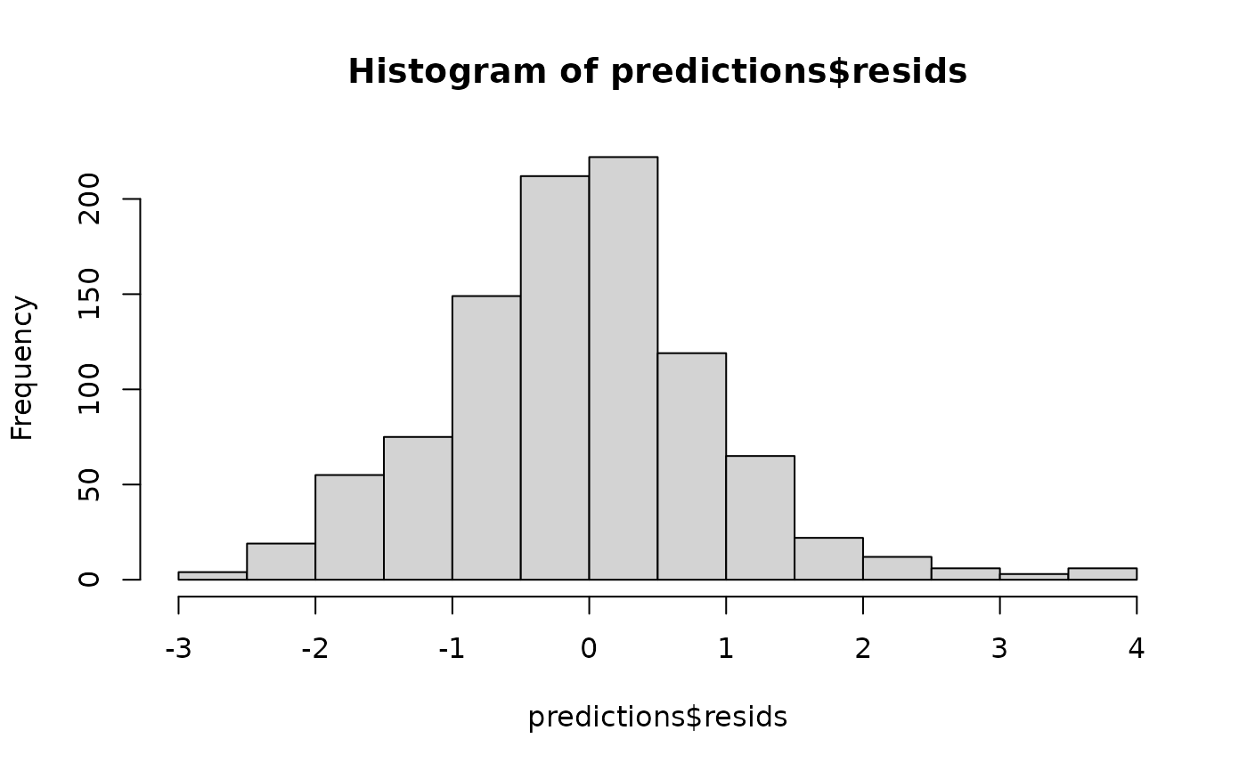
 hist(predictions$resids)
 qqnorm(predictions$resids);abline(a = 0, b = 1)
 # Predictions onto new data --------------------------------------------
qcs_grid_2011 <- replicate_df(qcs_grid, "year", unique(pcod_2011$year))
predictions <- predict(m, newdata = qcs_grid_2011)
# \donttest{
# A short function for plotting our predictions:
plot_map <- function(dat, column = est) {
ggplot(dat, aes(X, Y, fill = {{ column }})) +
geom_raster() +
facet_wrap(~year) +
coord_fixed()
}
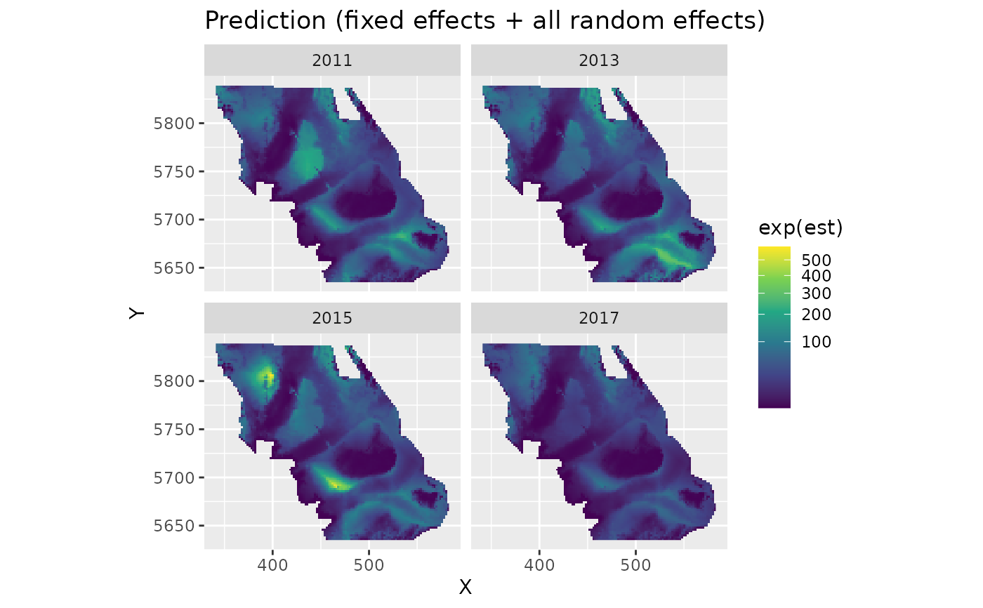
plot_map(predictions, exp(est)) +
scale_fill_viridis_c(trans = "sqrt") +
ggtitle("Prediction (fixed effects + all random effects)")
# Predictions onto new data --------------------------------------------
qcs_grid_2011 <- replicate_df(qcs_grid, "year", unique(pcod_2011$year))
predictions <- predict(m, newdata = qcs_grid_2011)
# \donttest{
# A short function for plotting our predictions:
plot_map <- function(dat, column = est) {
ggplot(dat, aes(X, Y, fill = {{ column }})) +
geom_raster() +
facet_wrap(~year) +
coord_fixed()
}
plot_map(predictions, exp(est)) +
scale_fill_viridis_c(trans = "sqrt") +
ggtitle("Prediction (fixed effects + all random effects)")
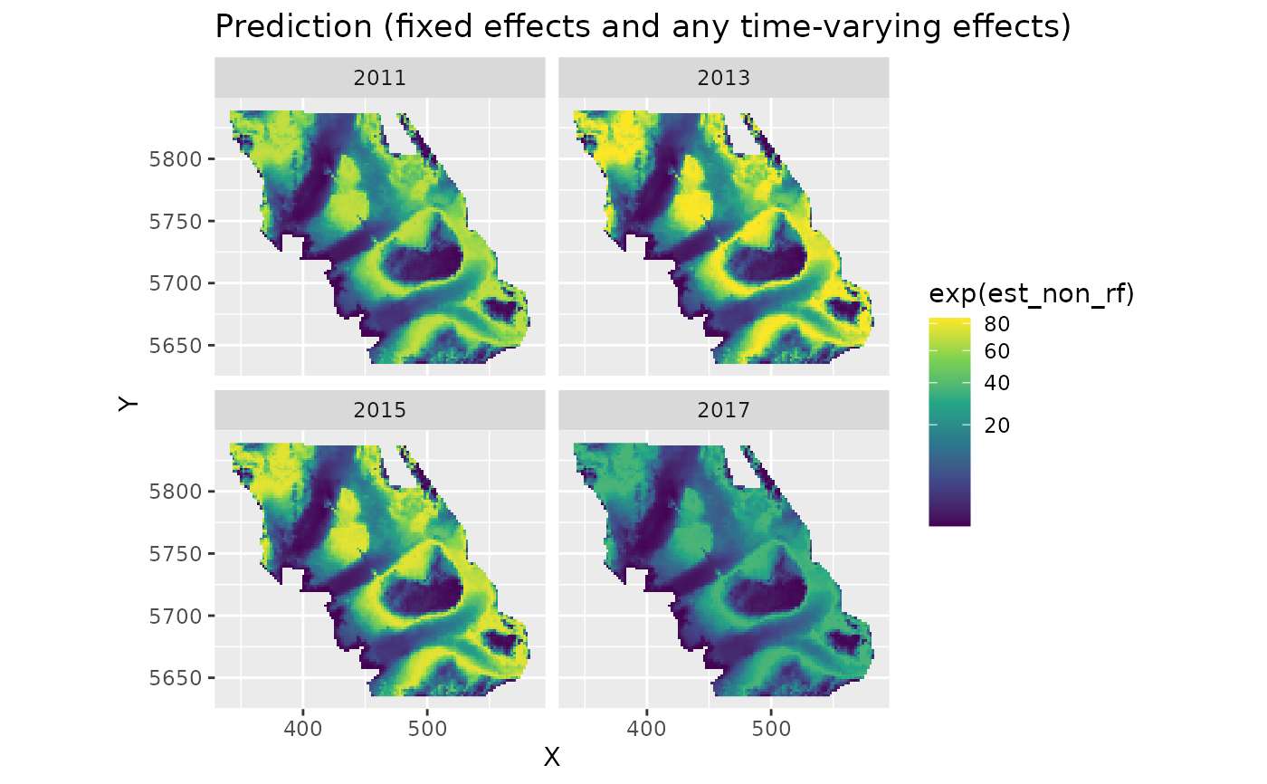
 plot_map(predictions, exp(est_non_rf)) +
ggtitle("Prediction (fixed effects and any time-varying effects)") +
scale_fill_viridis_c(trans = "sqrt")
plot_map(predictions, exp(est_non_rf)) +
ggtitle("Prediction (fixed effects and any time-varying effects)") +
scale_fill_viridis_c(trans = "sqrt")
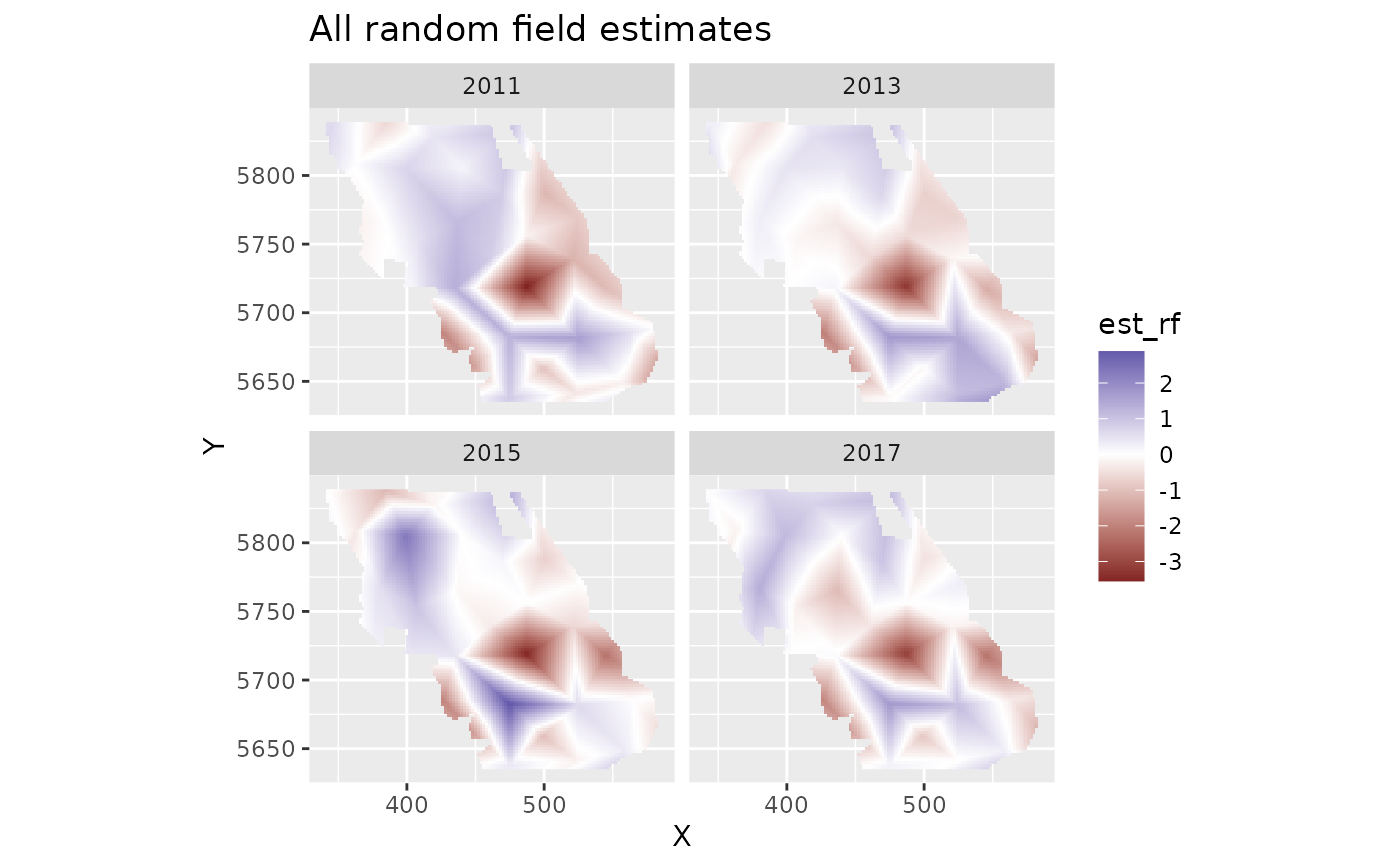
 plot_map(predictions, est_rf) +
ggtitle("All random field estimates") +
scale_fill_gradient2()
plot_map(predictions, est_rf) +
ggtitle("All random field estimates") +
scale_fill_gradient2()
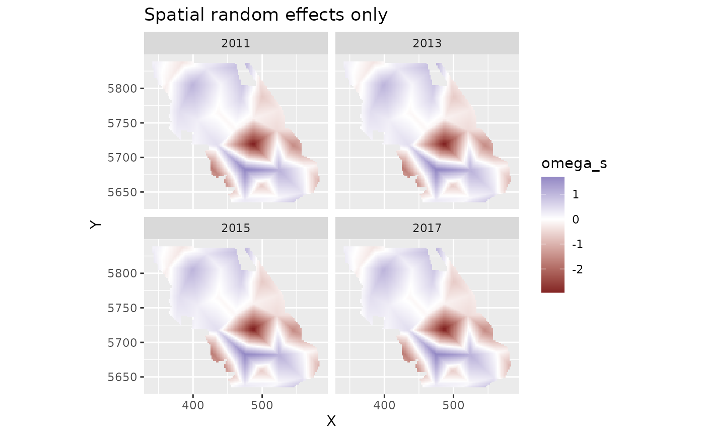
 plot_map(predictions, omega_s) +
ggtitle("Spatial random effects only") +
scale_fill_gradient2()
plot_map(predictions, omega_s) +
ggtitle("Spatial random effects only") +
scale_fill_gradient2()
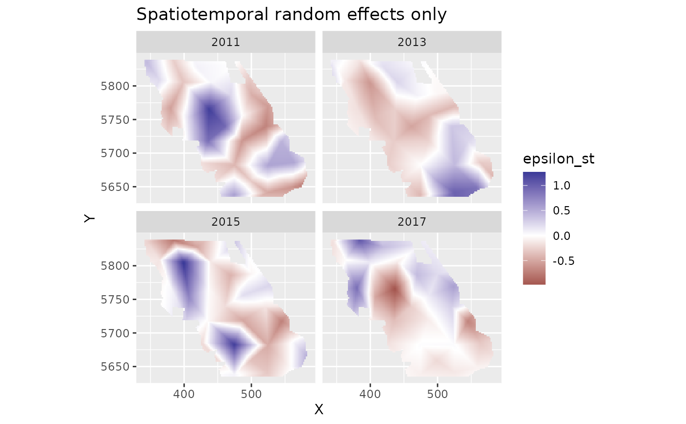
 plot_map(predictions, epsilon_st) +
ggtitle("Spatiotemporal random effects only") +
scale_fill_gradient2()
plot_map(predictions, epsilon_st) +
ggtitle("Spatiotemporal random effects only") +
scale_fill_gradient2()
 # Visualizing a marginal effect ----------------------------------------
# See the visreg package or the ggeffects::ggeffect() or
# ggeffects::ggpredict() functions
# To do this manually:
nd <- data.frame(depth_scaled =
seq(min(d$depth_scaled), max(d$depth_scaled), length.out = 100))
nd$depth_scaled2 <- nd$depth_scaled^2
# Because this is a spatiotemporal model, you'll need at least one time
# element. If time isn't also a fixed effect then it doesn't matter what you pick:
nd$year <- 2011L # L: integer to match original data
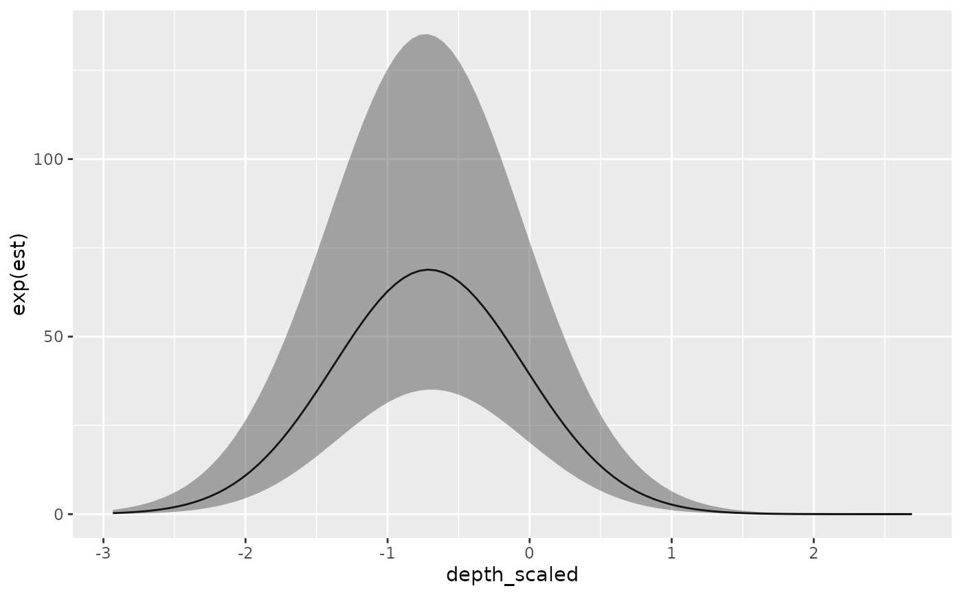
p <- predict(m, newdata = nd, se_fit = TRUE, re_form = NA)
ggplot(p, aes(depth_scaled, exp(est),
ymin = exp(est - 1.96 * est_se), ymax = exp(est + 1.96 * est_se))) +
geom_line() + geom_ribbon(alpha = 0.4)
# Visualizing a marginal effect ----------------------------------------
# See the visreg package or the ggeffects::ggeffect() or
# ggeffects::ggpredict() functions
# To do this manually:
nd <- data.frame(depth_scaled =
seq(min(d$depth_scaled), max(d$depth_scaled), length.out = 100))
nd$depth_scaled2 <- nd$depth_scaled^2
# Because this is a spatiotemporal model, you'll need at least one time
# element. If time isn't also a fixed effect then it doesn't matter what you pick:
nd$year <- 2011L # L: integer to match original data
p <- predict(m, newdata = nd, se_fit = TRUE, re_form = NA)
ggplot(p, aes(depth_scaled, exp(est),
ymin = exp(est - 1.96 * est_se), ymax = exp(est + 1.96 * est_se))) +
geom_line() + geom_ribbon(alpha = 0.4)
 # Plotting marginal effect of a spline ---------------------------------
m_gam <- sdmTMB(
data = d, formula = density ~ 0 + as.factor(year) + s(depth_scaled, k = 5),
time = "year", mesh = mesh, family = tweedie(link = "log")
)
if (require("visreg", quietly = TRUE)) {
visreg::visreg(m_gam, "depth_scaled")
}
# Plotting marginal effect of a spline ---------------------------------
m_gam <- sdmTMB(
data = d, formula = density ~ 0 + as.factor(year) + s(depth_scaled, k = 5),
time = "year", mesh = mesh, family = tweedie(link = "log")
)
if (require("visreg", quietly = TRUE)) {
visreg::visreg(m_gam, "depth_scaled")
}
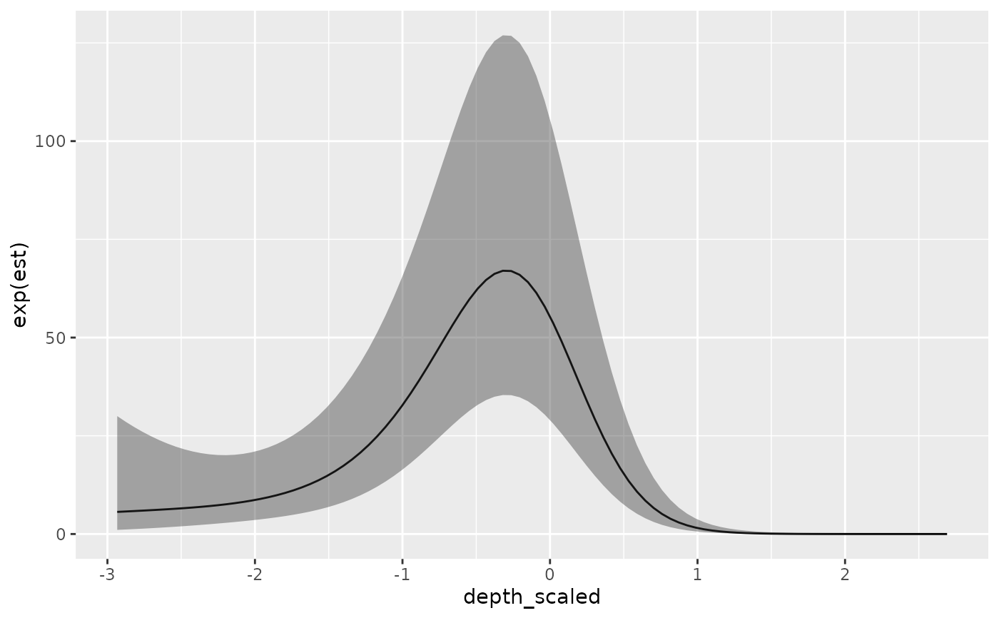
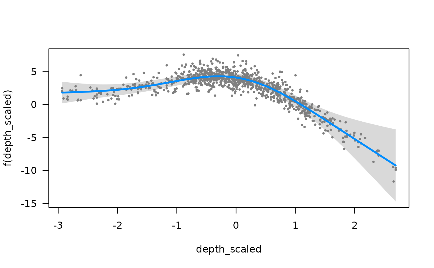 # or manually:
nd <- data.frame(depth_scaled =
seq(min(d$depth_scaled), max(d$depth_scaled), length.out = 100))
nd$year <- 2011L
p <- predict(m_gam, newdata = nd, se_fit = TRUE, re_form = NA)
ggplot(p, aes(depth_scaled, exp(est),
ymin = exp(est - 1.96 * est_se), ymax = exp(est + 1.96 * est_se))) +
geom_line() + geom_ribbon(alpha = 0.4)
# or manually:
nd <- data.frame(depth_scaled =
seq(min(d$depth_scaled), max(d$depth_scaled), length.out = 100))
nd$year <- 2011L
p <- predict(m_gam, newdata = nd, se_fit = TRUE, re_form = NA)
ggplot(p, aes(depth_scaled, exp(est),
ymin = exp(est - 1.96 * est_se), ymax = exp(est + 1.96 * est_se))) +
geom_line() + geom_ribbon(alpha = 0.4)
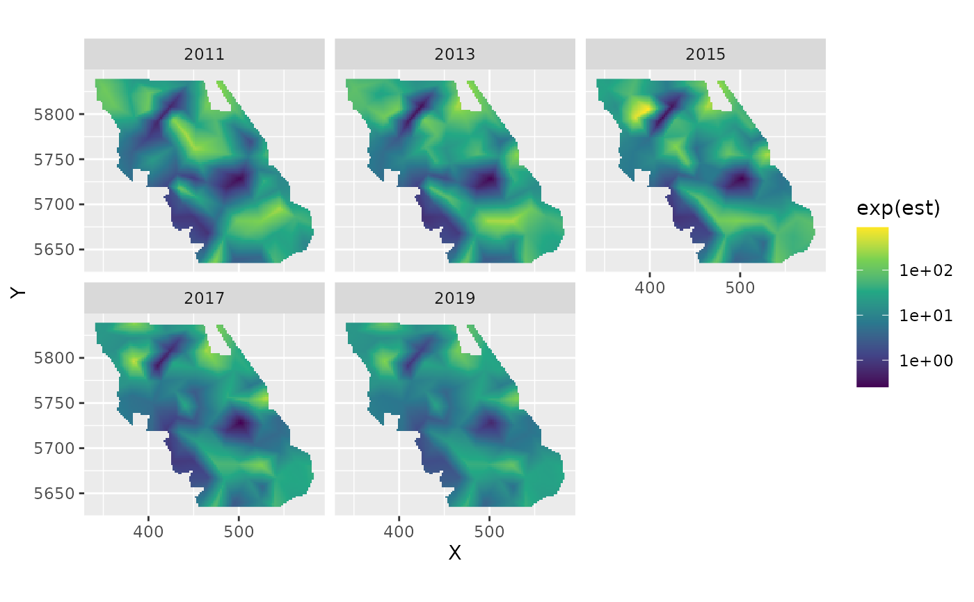
 # Forecasting ----------------------------------------------------------
mesh <- make_mesh(d, c("X", "Y"), cutoff = 15)
unique(d$year)
#> [1] 2011 2013 2015 2017
m <- sdmTMB(
data = d, formula = density ~ 1,
spatiotemporal = "AR1", # using an AR1 to have something to forecast with
extra_time = 2019L, # `L` for integer to match our data
spatial = "off",
time = "year", mesh = mesh, family = tweedie(link = "log")
)
# Add a year to our grid:
grid2019 <- qcs_grid_2011[qcs_grid_2011$year == max(qcs_grid_2011$year), ]
grid2019$year <- 2019L # `L` because `year` is an integer in the data
qcsgrid_forecast <- rbind(qcs_grid_2011, grid2019)
predictions <- predict(m, newdata = qcsgrid_forecast)
plot_map(predictions, exp(est)) +
scale_fill_viridis_c(trans = "log10")
# Forecasting ----------------------------------------------------------
mesh <- make_mesh(d, c("X", "Y"), cutoff = 15)
unique(d$year)
#> [1] 2011 2013 2015 2017
m <- sdmTMB(
data = d, formula = density ~ 1,
spatiotemporal = "AR1", # using an AR1 to have something to forecast with
extra_time = 2019L, # `L` for integer to match our data
spatial = "off",
time = "year", mesh = mesh, family = tweedie(link = "log")
)
# Add a year to our grid:
grid2019 <- qcs_grid_2011[qcs_grid_2011$year == max(qcs_grid_2011$year), ]
grid2019$year <- 2019L # `L` because `year` is an integer in the data
qcsgrid_forecast <- rbind(qcs_grid_2011, grid2019)
predictions <- predict(m, newdata = qcsgrid_forecast)
plot_map(predictions, exp(est)) +
scale_fill_viridis_c(trans = "log10")
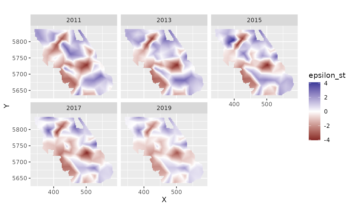
 plot_map(predictions, epsilon_st) +
scale_fill_gradient2()
plot_map(predictions, epsilon_st) +
scale_fill_gradient2()
 # Estimating local trends ----------------------------------------------
d <- pcod
d$year_scaled <- as.numeric(scale(d$year))
mesh <- make_mesh(pcod, c("X", "Y"), cutoff = 25)
m <- sdmTMB(data = d, formula = density ~ depth_scaled + depth_scaled2,
mesh = mesh, family = tweedie(link = "log"),
spatial_varying = ~ 0 + year_scaled, time = "year", spatiotemporal = "off")
nd <- replicate_df(qcs_grid, "year", unique(pcod$year))
nd$year_scaled <- (nd$year - mean(d$year)) / sd(d$year)
p <- predict(m, newdata = nd)
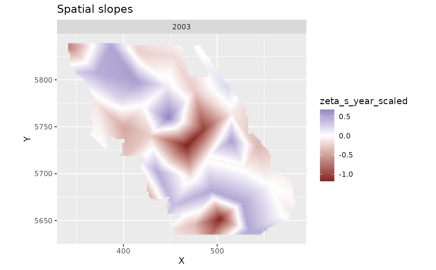
plot_map(subset(p, year == 2003), zeta_s_year_scaled) + # pick any year
ggtitle("Spatial slopes") +
scale_fill_gradient2()
# Estimating local trends ----------------------------------------------
d <- pcod
d$year_scaled <- as.numeric(scale(d$year))
mesh <- make_mesh(pcod, c("X", "Y"), cutoff = 25)
m <- sdmTMB(data = d, formula = density ~ depth_scaled + depth_scaled2,
mesh = mesh, family = tweedie(link = "log"),
spatial_varying = ~ 0 + year_scaled, time = "year", spatiotemporal = "off")
nd <- replicate_df(qcs_grid, "year", unique(pcod$year))
nd$year_scaled <- (nd$year - mean(d$year)) / sd(d$year)
p <- predict(m, newdata = nd)
plot_map(subset(p, year == 2003), zeta_s_year_scaled) + # pick any year
ggtitle("Spatial slopes") +
scale_fill_gradient2()
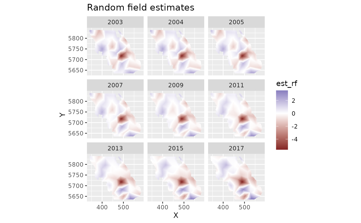
 plot_map(p, est_rf) +
ggtitle("Random field estimates") +
scale_fill_gradient2()
plot_map(p, est_rf) +
ggtitle("Random field estimates") +
scale_fill_gradient2()
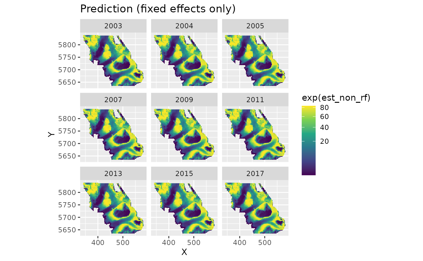
 plot_map(p, exp(est_non_rf)) +
ggtitle("Prediction (fixed effects only)") +
scale_fill_viridis_c(trans = "sqrt")
plot_map(p, exp(est_non_rf)) +
ggtitle("Prediction (fixed effects only)") +
scale_fill_viridis_c(trans = "sqrt")
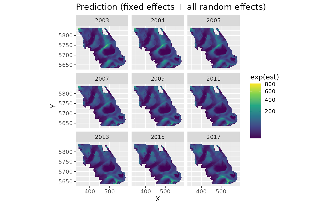
 plot_map(p, exp(est)) +
ggtitle("Prediction (fixed effects + all random effects)") +
scale_fill_viridis_c(trans = "sqrt")
plot_map(p, exp(est)) +
ggtitle("Prediction (fixed effects + all random effects)") +
scale_fill_viridis_c(trans = "sqrt")
 # }
# }