Fitting multispecies models with sdmTMB

If the code in this vignette has not been evaluated, a rendered version is available on the documentation site under ‘Articles’.

library(sdmTMB)

For some applications, we might be interested in fitting a model that includes multiple responses such as 2+ species, or multiple size or age classes within a species. The most important step in fitting these models is understanding which parameters are shared, and which parameters are species-specific.

Below, we illustrate a series of models. We’ll start by simulating a 2-species dataset. Each species is allowed to have unique spatial standard deviations (sigma_O) as well as different year effects.

set.seed(1)
predictor_dat <- data.frame(
  X = runif(1000), Y = runif(1000),
  year = rep(1:5, each = 200)
)
predictor_dat$fyear <- as.factor(predictor_dat$year)
mesh <- make_mesh(predictor_dat, xy_cols = c("X", "Y"), cutoff = 0.1)
sim_dat_A <- sdmTMB_simulate(
  formula = ~ 0 + fyear,
  data = predictor_dat,
  time = "year",
  mesh = mesh,
  range = 0.2,
  family = gaussian(),
  seed = 42,
  sigma_O = 0.2,
  phi = 0.1,
  sigma_E = 0.3,
  B = runif(5, min = 5, max = 8) # 5 random year effects
)
sim_dat_A$species <- "A"
sim_dat_B <- sdmTMB_simulate(
  formula = ~ 0 + fyear,
  data = predictor_dat,
  time = "year",
  mesh = mesh,
  range = 0.2,
  family = gaussian(),
  seed = 43,
  sigma_O = 0.3,
  phi = 0.1,
  sigma_E = 0.3,
  B = runif(5, min = 5, max = 8) # 5 random year effects
)
sim_dat_B$species <- "B"
sim_dat <- rbind(sim_dat_A, sim_dat_B)
sim_dat$fyear <- factor(sim_dat$year)

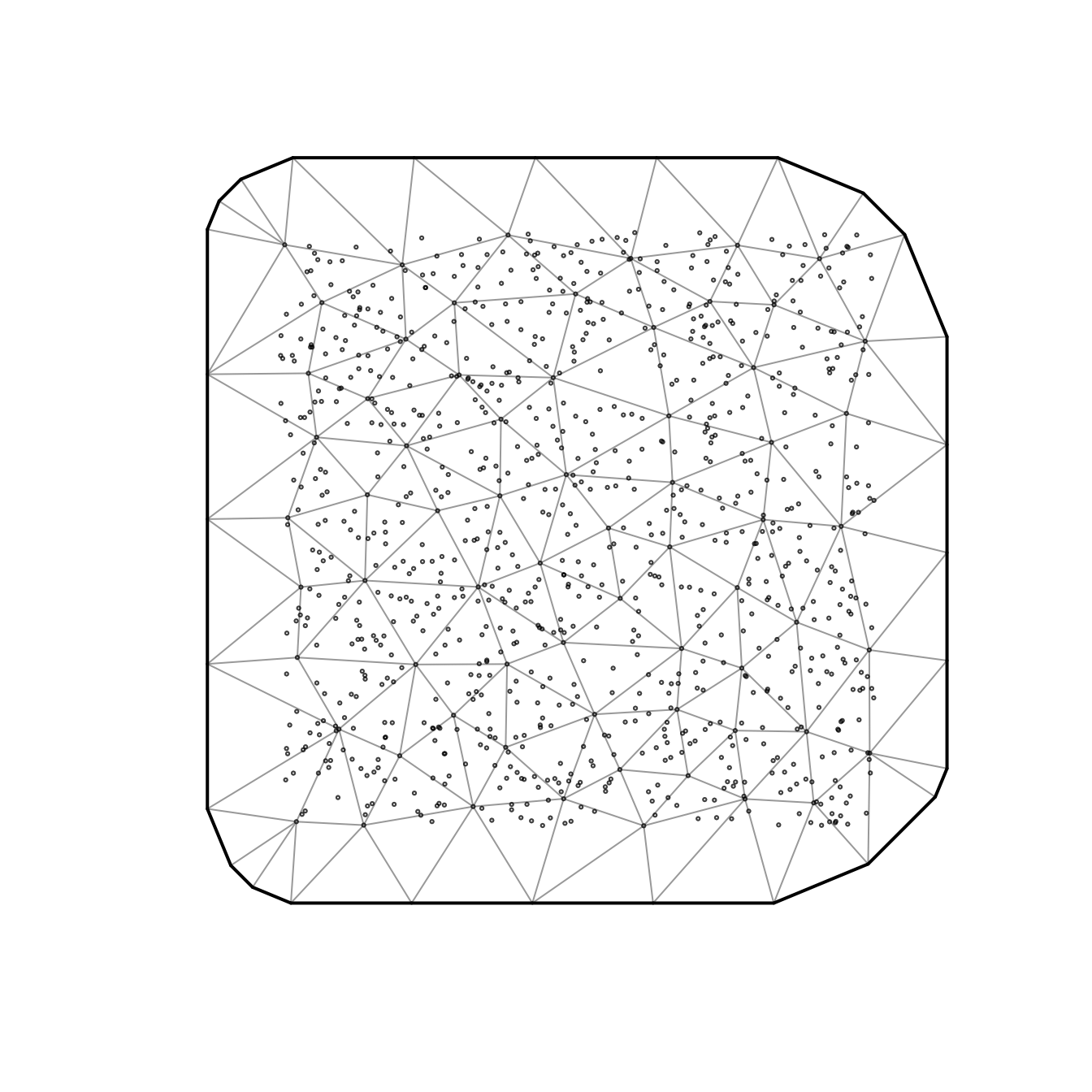
We’ll start by making an SPDE mesh across the full dataset.

mesh <- make_mesh(sim_dat, c("X", "Y"), cutoff = 0.1)
plot(mesh)

Model 1: species-specific intercepts

As a first model, we can include species-specific year effects. This can be done in a couple ways. One option would be to estimate the species * year interaction, letting the year effects for each species be independent. Here, all other parameters and random effect values (range, spatial field, spatial variance, spatiotemporal fields, spatiotemporal variances) are shared.

fit <- sdmTMB(
  observed ~ fyear * species,
  data = sim_dat,
  time = "year",
  spatiotemporal = "iid",
  mesh = mesh,
  family = gaussian()
)
fit
#> Spatiotemporal model fit by ML ['sdmTMB']
#> Formula: observed ~ fyear * species
#> Mesh: mesh (isotropic covariance)
#> Time column: year
#> Data: sim_dat
#> Family: gaussian(link = 'identity')
#>  
#>                 coef.est coef.se
#> (Intercept)         7.59    0.05
#> fyear2              0.36    0.05
#> fyear3              0.02    0.05
#> fyear4             -1.19    0.05
#> fyear5             -1.93    0.05
#> speciesB           -1.49    0.03
#> fyear2:speciesB     0.02    0.04
#> fyear3:speciesB    -0.71    0.04
#> fyear4:speciesB     0.70    0.04
#> fyear5:speciesB     3.45    0.04
#> 
#> Dispersion parameter: 0.27
#> Matérn range: 0.19
#> Spatial SD: 0.17
#> Spatiotemporal IID SD: 0.14
#> ML criterion at convergence: 329.263
#> 
#> See ?tidy.sdmTMB to extract these values as a data frame.

Model 2: species-specific spatial fields

We may be interested in fitting a model that lets the spatial patterning differ by species. These kinds of models can be expressed using spatially varying coefficients. Note that we use spatial = off because this represents a global spatial intercept—turning this off is akin to using a -1 of 0 in a main formula including a factor. Both species take their spatial fields from the spatial_varying field here.

fit <- sdmTMB(
  observed ~ fyear * species,
  data = sim_dat,
  mesh = mesh,
  family = gaussian(),
  spatial = "off",
  time = "year",
  spatiotemporal = "iid",
  spatial_varying = ~ 0 + factor(species)
)
fit
#> Spatiotemporal model fit by ML ['sdmTMB']
#> Formula: observed ~ fyear * species
#> Mesh: mesh (isotropic covariance)
#> Time column: year
#> Data: sim_dat
#> Family: gaussian(link = 'identity')
#>  
#>                 coef.est coef.se
#> (Intercept)         7.60    0.06
#> fyear2              0.36    0.05
#> fyear3              0.04    0.05
#> fyear4             -1.22    0.05
#> fyear5             -1.94    0.05
#> speciesB           -1.51    0.08
#> fyear2:speciesB     0.02    0.03
#> fyear3:speciesB    -0.75    0.03
#> fyear4:speciesB     0.76    0.03
#> fyear5:speciesB     3.48    0.03
#> 
#> Dispersion parameter: 0.19
#> Matérn range: 0.18
#> Spatially varying coefficient SD (factor(species)A): 0.25
#> Spatially varying coefficient SD (factor(species)B): 0.30
#> Spatiotemporal IID SD: 0.16
#> ML criterion at convergence: -170.949
#> 
#> See ?tidy.sdmTMB to extract these values as a data frame.

You’ll notice that there are two rows of entries for sigma_Z our spatially varying random field standard deviation:

tidy(fit, "ran_pars")
#> # A tibble: 5 × 5
#>   term    estimate std.error conf.low conf.high
#>   <chr>      <dbl>     <dbl>    <dbl>     <dbl>
#> 1 range      0.181   0.0250     0.139     0.238
#> 2 phi        0.189   0.00330    0.183     0.195
#> 3 sigma_E    0.162   0.0129     0.139     0.190
#> 4 sigma_Z    0.250   0.0268     0.203     0.308
#> 5 sigma_Z    0.302   0.0303     0.248     0.367

This means that our model is trying to estimate separate species-specific variance terms for the species-specific spatial fields (say that 10 times fast!). Here, that matches how we simulated the data. In other contexts, especially if we ran into estimation issues, we might want to share those SDs.

If we wanted to estimate species-specific spatial fields with a single shared variance (meaning the net magnitude of the peaks and valleys in the fields were similar but the wiggles themselves were species specific), we could do that by specifying a custom map argument and passing it into sdmTMBcontrol(). Any shared factor levels in the map are gathered to have ‘mirrored’ or shared parameter values. We assign these to ln_tau_Z because, internally, this is the parameter that gets converted into the spatially-varying field variances (the SDs of those fields are sigma_Z).

This case is pretty simple, but for more complicated cases we could figure out the structure of our needed map vector as follows:

colnames(model.matrix(~ 0 + factor(species), data = sim_dat))
#> [1] "factor(species)A" "factor(species)B"

So, we need a vector of length two with shared factor values:

map_list <- list(ln_tau_Z = factor(c(1, 1)))

Then, we can use our map list to share the spatially varying coefficient SDs:

fit <- sdmTMB(
  observed ~ fyear * factor(species),
  data = sim_dat,
  mesh = mesh,
  family = gaussian(),
  spatial = "off",
  time = "year",
  spatiotemporal = "iid",
  spatial_varying = ~ 0 + factor(species),
  control = sdmTMBcontrol(map = map_list)
)
fit
#> Spatiotemporal model fit by ML ['sdmTMB']
#> Formula: observed ~ fyear * factor(species)
#> Mesh: mesh (isotropic covariance)
#> Time column: year
#> Data: sim_dat
#> Family: gaussian(link = 'identity')
#>  
#>                         coef.est coef.se
#> (Intercept)                 7.60    0.06
#> fyear2                      0.35    0.05
#> fyear3                      0.04    0.05
#> fyear4                     -1.23    0.05
#> fyear5                     -1.94    0.05
#> factor(species)B           -1.51    0.08
#> fyear2:factor(species)B     0.02    0.03
#> fyear3:factor(species)B    -0.75    0.03
#> fyear4:factor(species)B     0.76    0.03
#> fyear5:factor(species)B     3.48    0.03
#> 
#> Dispersion parameter: 0.19
#> Matérn range: 0.18
#> Spatially varying coefficient SD (factor(species)A): 0.28
#> Spatially varying coefficient SD (factor(species)B): 0.28
#> Spatiotemporal IID SD: 0.16
#> ML criterion at convergence: -170.110
#> 
#> See ?tidy.sdmTMB to extract these values as a data frame.

Notice the spatially varying coefficient SD is now shared.

Model 3: species-specific spatiotemporal fields

In all of the examples above, spatiotemporal fields are included, but shared among species. As another example, we can extend the above approaches to set up a model that includes spatiotemporal fields unique to each species.

One approach to including separate spatiotemporal fields by species is creating a new variable that is a concatenation of species and year (or any given time step factor). For example, we can then implement this form of species-specific spatiotemporal variation by changing the time argument to be time = "species_year".

sim_dat$species_year <- factor(paste(sim_dat$species, sim_dat$year))
map_list <- list(ln_tau_Z = factor(c(1, 1)))
fit <- sdmTMB(
  observed ~ fyear * factor(species),
  data = sim_dat,
  mesh = mesh,
  family = gaussian(),
  spatial = "off",
  time = "species_year",
  spatiotemporal = "iid",
  spatial_varying = ~ 0 + factor(species),
  control = sdmTMBcontrol(map = map_list)
)
fit
#> Spatiotemporal model fit by ML ['sdmTMB']
#> Formula: observed ~ fyear * factor(species)
#> Mesh: mesh (isotropic covariance)
#> Time column: species_year
#> Data: sim_dat
#> Family: gaussian(link = 'identity')
#>  
#>                         coef.est coef.se
#> (Intercept)                 7.56    0.07
#> fyear2                      0.38    0.08
#> fyear3                      0.06    0.08
#> fyear4                     -1.19    0.08
#> fyear5                     -1.92    0.08
#> factor(species)B           -1.43    0.10
#> fyear2:factor(species)B    -0.03    0.11
#> fyear3:factor(species)B    -0.79    0.11
#> fyear4:factor(species)B     0.67    0.11
#> fyear5:factor(species)B     3.42    0.11
#> 
#> Dispersion parameter: 0.10
#> Matérn range: 0.16
#> Spatially varying coefficient SD (factor(species)A): 0.25
#> Spatially varying coefficient SD (factor(species)B): 0.25
#> Spatiotemporal IID SD: 0.31
#> ML criterion at convergence: -917.518
#> 
#> See ?tidy.sdmTMB to extract these values as a data frame.

Model 4: hack species into the time element for spatial models

If we only wanted to fit a spatial model but had several species (or other groups), one approach is to pretend our species (or other group) is the time element.

sim_dat$numeric_species <- as.numeric(factor(sim_dat$species)) # needs to be numeric
fit_fake_time <- sdmTMB(
  observed ~ 0 + factor(species),
  data = sim_dat,
  mesh = mesh,
  family = gaussian(),
  spatial = "off",
  time = "numeric_species", #< hack
  spatiotemporal = "iid" #< 'AR1' or 'RW' probably wouldn't make sense here
)
fit_fake_time
#> Spatiotemporal model fit by ML ['sdmTMB']
#> Formula: observed ~ 0 + factor(species)
#> Mesh: mesh (isotropic covariance)
#> Time column: numeric_species
#> Data: sim_dat
#> Family: gaussian(link = 'identity')
#>  
#>                  coef.est coef.se
#> factor(species)A     7.01    0.08
#> factor(species)B     6.27    0.08
#> 
#> Dispersion parameter: 0.86
#> Matérn range: 0.33
#> Spatiotemporal IID SD: 0.21
#> ML criterion at convergence: 2568.873
#> 
#> See ?tidy.sdmTMB to extract these values as a data frame.

This is just a convenience though. We could instead do the same thing using the spatial_varying argument making sure to ‘map’ the field variances to be shared to match the above:

fit_svc <- sdmTMB(
  observed ~ 0 + factor(species),
  data = sim_dat,
  mesh = mesh,
  family = gaussian(),
  spatial = "off",
  spatial_varying = ~ 0 + factor(species),
  control = sdmTMBcontrol(map = list(ln_tau_Z = factor(c(1, 1))))
)
fit_svc
#> Spatial model fit by ML ['sdmTMB']
#> Formula: observed ~ 0 + factor(species)
#> Mesh: mesh (isotropic covariance)
#> Data: sim_dat
#> Family: gaussian(link = 'identity')
#>  
#>                  coef.est coef.se
#> factor(species)A     7.01    0.08
#> factor(species)B     6.27    0.08
#> 
#> Dispersion parameter: 0.86
#> Matérn range: 0.33
#> Spatially varying coefficient SD (factor(species)A): 0.21
#> Spatially varying coefficient SD (factor(species)B): 0.21
#> ML criterion at convergence: 2568.873
#> 
#> See ?tidy.sdmTMB to extract these values as a data frame.

We can prove they’re identical:

logLik(fit_fake_time)
#> 'log Lik.' -2568.873 (df=5)
logLik(fit_svc)
#> 'log Lik.' -2568.873 (df=5)

Putting it all together

These examples illustrate a number of ways that species-specific effects can be included in sdmTMB models, and can be extended to other categories/groups/cohorts within a species for which one wants to control the amount of information shared between groups (e.g., age-, size-, or stage-specific estimates). A brief summary of these approaches can be summarized as:

Form	Implementation
Main effects	Year-by-species interactions or smooths by year
Spatial effects	Spatially varying coefficients
Spatial effects w/shared variance	Spatially varying coefficients + map argument
Spatiotemporal effects	Species-year factor as time variable

Further extensions